To Run & Understand The "Suspension System Comparison"

AIM:-
To Plot a function y(x) = (x-1) * (x-3)^2 * (x-9)^2
To Run Simulink example For “Suspension System Comparison”

#PART 1
To Plot a function y(x) = (x-1) * (x-3)^2 * (x-9)^2

Governing Equation:-
y(x) = (x-1) * (x-3)^2 * (x-9)^2

Objective:-
To Plot a function y(x) = (x-1) * (x-3)^2 * (x-9)^2 using basic Simulink blocks.

BODY OF THE CONTENT:-
The function y(x) is a basic Mathematical Function, which can be built on Simulink using basic Simulink blocks. The value of 'x' is independent and was given by using 'Ramp', which varied with respect to the time given to run the simulation. The time given to run the simulation is 10second, and the slope is 1.

Input- Simulink Model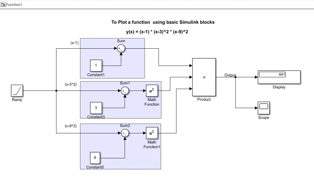

Basic Simulink blocks used-
Ramp- The Ramp block generates a signal that starts at a specified time and value and changes by a specified rate.
Constant- The Constant block generates a real or complex constant value signal. Use this block to provide a constant signal input. The block generates scalar, vector, or matrix output, depending on
Sum- The Sum block performs addition or subtraction on its inputs.
Math Function- Math Function block performs numerous common mathematical functions
Product- Multiply and divide scalars and nonscalars or multiply and invert matrices
Display- The Display block shows the value of the input data
Scope- Display signals generated during simulation

Output-

Display-The Output observed after the end of the simulation on Display Block is 441.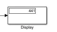

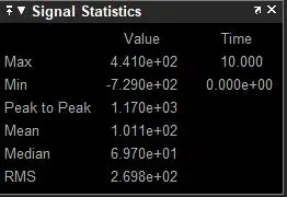
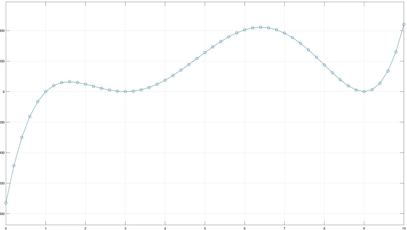
Scope- The Graph Plots in the Scope Block after the simulation calculated the function y(x) at each point, the Range of the points plotted in 10second on Graph is -729 to 441

#PART 2-
To Run Simulink example For “Suspension System Comparison”

Objective:-

1. On the basis of the Study For “Suspension System Comparison” answer the following,

• What is the objective of the simulation? What are the similarities and differences between the three systems understudy?
• What are your observations from the results?
• How the oscillating velocity source is created?

BODY OF THE CONTENT:-
Simulink model for “Suspension System Comparison” can be found in the Simulink Help Document.
The objective of the study is to understand the behavior of three suspension systems under one excitation source and how they behave on similar oscillation velocity.

Theory- This example shows a testbed containing three sets of springs and dampers excited by the same oscillating velocity source. The first uses the Shock Absorber block and includes linear stiffness and damping. The second shock absorber uses a Nonlinear Translational Spring and a Nonlinear Translational Damper specified by symmetric polynomials. The third uses a Variable Translational Spring and Variable Translational Damper.
The arrangement is done to improve the quality of driving in a vehicle.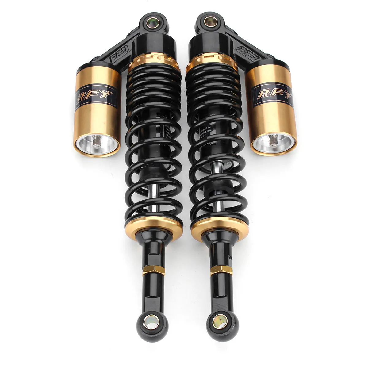

Shock Absorber- A shock absorber or damper is a mechanical or hydraulic device designed to absorb and damp shock impulses In a vehicle, shock absorbers reduce the effect of traveling over rough ground, leading to improved ride quality and vehicle handling.

Objective of the simulation:-
Simulation is a data flow graphical programming language tool for modeling, simulating, and analyzing multi-domain dynamic systems. It is basically a graphical block diagramming tool with a customizable set of block libraries.

1. Risk-free environment- Simulation modeling provides a safe way to test and explore different “what-if” scenarios. The effect of changing staffing levels in a plant may be seen without putting production at risk. Make the right decision before making real-world changes.
2. Save money and time- Virtual experiments with simulation models are less expensive and take less time than experiments with real assets.
3. Visualization- Simulation models can be animated in 2D/3D, allowing concepts and ideas to be more easily verified, communicated, and understood. Analysts and engineers gain trust in a model by seeing it in action and can clearly demonstrate findings to management.
4. Increased accuracy- A simulation model can capture many more details than an analytical model, providing increased accuracy and more precise forecasting.

Similarities and Differences between the Three Systems Understudy

- Velocity source applied as the same input for all three systems.
- Tire stiffness, sprung mass and unsprung mass are similar for all three systems.
- The spring and damping parameters are different in each setup.,
- Fist setup of this system includes linear stiffness and damping. optional friction and hard stops are not used
- The second setup of shock absorber includes a non-linear translational spring and non-linear translational damper, which is specified with a symmetric polynomial.
- The third setup includes a variable translational spring and a variable translational damper, the spring constant varies during the simulation, and the damping coefficient adjusts to achieve critical damping.

INPUT:-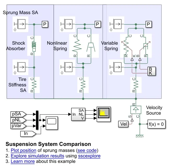

OUTPUT:-
Result 1- Sprung Mass Position & Input Velocity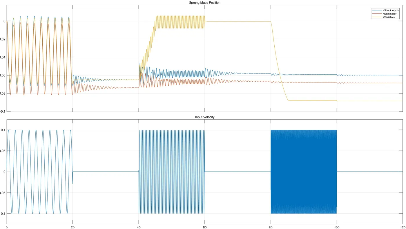

Observation from the result:-
Here from the graph, it is shown, as we applied input oscillating frequency 3rad/sec to a time period of 0-20sec, in all three systems, the position of sprung mass is almost the same.
After increasing the input oscillating frequency to 15rad/sec for a time period between 40-60 sec, the variable setup oscillation of the sprung mass experience minimal vibration, whereas the linear and non-linear setups experience high vibrations.
On increasing the input oscillating frequency to 75rad/sec for time lap 80-100sec, the variable transitional spring damper setup adjusted the sprung mass position tp -0.9m with minimum vibration, whereas the linear transitional spring damper setup and non-linear transitional spring damper setup adjusted to sprung mass around -0.6m and -0.7m respectively.
But it has more vibration in linear and non-linear comparatively variable setup.

Result 2- Power Spectral Velocity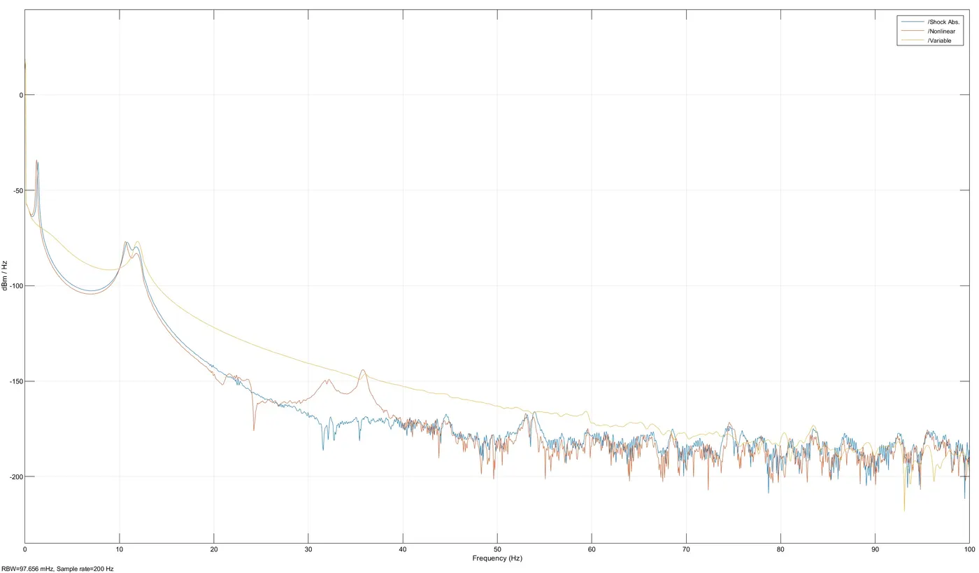

Oscillating velocity source:-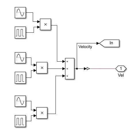

- The Oscillating velocity source is created using the three Sinewave(with three Different frequency 3rad/sec, 15rad/sec, 75rad/sec respectively ) & three Pulse Generator blocks.
- The time period for each oscillation is given as 20seconds, with a time delay of 20second
- The output of all these sine and Pulse Generator blocks are multiplied and then added to generate the velocity signal.


Conclusion:-
- We can use the Constant block and assign values to 'x' and get the output.
- Ramp block can be used to give variable inputs to the function.
- On comparing all system, the shock absorber spring damper setup seems good stiffness, vibration is low in this setup.
- The non-linear spring-damper setup is the same as the linear spring-damper setup but the stiffness is low comparatively
- The variable spring damper setup seems bad performance, on change in frequency, sudden highs and falls occurred, so considered as the poor system.