Structural dynamics

1.Differentiate Static analysis and Dynamic analysis with proper representing pictures

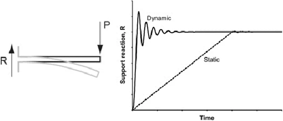
_{Static Analysis in Structural Dynamics}

• _{Definition: Static analysis in structural dynamics involves evaluating structures under static or quasi-static loads, assuming the loads are applied slowly enough that dynamic effects (like inertia and damping) can be ignored.}
• _{When it's performed: Typically used for assessing the structural integrity under constant or slowly varying loads.}
• _{Tools: Finite element analysis (FEA) software (e.g., ANSYS, Abaqus).}
• _{Applications: Buildings under constant loads (like weight), bridges under steady traffic, dams, and other static structures.}
• _Advantages:
  • _{Simpler and less computationally intensive than dynamic analysis.}
  • _{Provides a clear understanding of stress, strain, and displacement under static conditions.}
• _{Disadvantages:}
  • _{Does not account for time-dependent effects, inertia, or damping.}
  • _{Inaccurate for structures subjected to rapidly changing loads.}

_{Dynamic Analysis in Structural Dynamics}

• _{Definition: Dynamic analysis evaluates structures under loads that vary with time, accounting for inertia, damping, and other dynamic effects.}
• _{When it's performed: Used when structures are subjected to time-varying or impulsive loads, such as earthquakes, wind loads, and vibrations.}
• _{Tools: FEA software with dynamic analysis capabilities (e.g., ANSYS, Abaqus, SAP2000).}
• _{Applications: Earthquake engineering, wind turbine design, vehicle crash analysis, and vibration analysis of machinery.}
• _Advantages:
  • _{Provides a comprehensive understanding of structural behavior under dynamic loads.}
  • _{Essential for ensuring safety and performance in scenarios where loads change rapidly.}
• _{Disadvantages:}
• _{More complex and computationally intensive than static analysis.}
• _{Requires detailed information about the dynamic properties of materials and damping characteristics.}

2. Explain the following with relevant force-displacement graph

1. Elastic behavior
2. Inelastic behavior
3. Plastic behavior
4. Non-linear Inelastic behavior

Understanding different types of material behavior under load is crucial in structural dynamics and materials science. Each type of behavior can be illustrated with a force-displacement graph, which shows how a material deforms under applied forces. Let's explain each behavior with the corresponding force-displacement graph.

1. Elastic Behavior

Definition: Elastic behavior is when a material deforms under load but returns to its original shape when the load is removed. The deformation is reversible and proportional to the applied load.

Graph Characteristics:

The graph is a straight line, indicating a linear relationship between force and displacement.

The slope of the line is the material's stiffness or Young's modulus.

No permanent deformation occurs.

Force

^

|

| Elastic Behavior

| /

| /

| /

| /

| /

| /

| /

| /______________________> Displacement

2. Inelastic Behavior

Definition: Inelastic behavior occurs when the material does not return to its original shape after the load is removed. It includes both elastic and plastic deformation components.

Graph Characteristics:

The graph initially follows a linear path (elastic region) and then deviates into a non-linear path.

When the load is removed, the material does not return to zero displacement, indicating permanent deformation.

Force

^

|

| Inelastic Behavior

| /

| /

| / Elastic

| /__________

| / \

| / \_____

| / \ Inelastic

| /_____________________\__________________> Displacement

3. Plastic Behavior

Definition: Plastic behavior is a type of inelastic behavior where the material undergoes permanent deformation after yielding, even when the load is removed.

Graph Characteristics:

The graph starts with a linear elastic region, followed by a yield point where permanent deformation begins.

Beyond the yield point, the material deforms plastically.

The unloading path is parallel to the initial elastic line, but it does not return to the original zero displacement.

Force

^

|

| Plastic Behavior

| /

| /

| / Elastic

| /__________

| / \

| / \_____

| / \ Plastic

| / \

|/_______________________\________________> Displacement

4. Non-linear Inelastic Behavior

Definition: Non-linear inelastic behavior involves complex deformation where the material response is neither perfectly elastic nor purely plastic. It includes non-linear elasticity, plasticity, and potential other time-dependent behaviors like viscoelasticity or creep.

Graph Characteristics:

The initial part of the graph may be non-linear, indicating non-linear elasticity.

After yielding, the curve becomes more complex and does not follow a simple linear or plastic path.

The unloading path can be different from the loading path, showing hysteresis.

Force

^

|

| Non-linear Inelastic Behavior

| /

| /

| /

| /

| / Non-linear

| / Elastic

| /

| /

|/_____________________

| \

| \

| \

| \ Non-linear Inelastic

| \__________________> Displacement

Summary

Elastic Behavior: Linear and reversible deformation.

Inelastic Behavior: Combination of elastic and permanent deformation.

Plastic Behavior: Permanent deformation after yield point.

Non-linear Inelastic Behavior: Complex deformation involving non-linear elasticity and plasticity, often with hysteresis.

These graphs visually represent how materials respond to applied forces, helping in understanding their behavior under different loading conditions.

3. Explain Mass, Stiffness & Damping components in the equation of motion

In the context of mechanical vibrations and dynamics, the equation of motion typically describes the behavior of a system under various forces. For a single degree of freedom (SDOF) system, the equation of motion is often expressed as:

$m\ddot{x}(t) + c\dot{x}(t) + kx(t) = F(t)$mx¨(t)+cx˙(t)+kx(t)=F(t)

where:

• $m$m is the mass of the system,
• $c$c is the damping coefficient,
• $k$k is the stiffness of the system,
• $x(t)$x(t) is the displacement as a function of time,
• $\dot{x}(t)$x˙(t) is the velocity,
• $\ddot{x}(t)$x¨(t) is the acceleration,
• $F(t)$F(t) is the external force applied to the system.

Mass ( $m$m )

The mass represents the inertia of the system. It quantifies the resistance of the system to changes in its motion. In the equation of motion, the term $m\ddot{x}(t)$mx¨(t) corresponds to the inertial force, which is proportional to the acceleration. The greater the mass, the larger the force needed to achieve a given acceleration.

Stiffness ( $k$k )

The stiffness of the system is a measure of its resistance to deformation. It defines the relationship between the applied force and the resulting displacement. The term $kx(t)$kx(t) in the equation represents the restoring force that is proportional to the displacement. A stiffer system (with a higher $k$k value) will deform less under the same applied force, leading to a larger restoring force for a given displacement.

Damping ( $c$c )

Damping represents the dissipative forces that oppose the motion of the system, typically due to friction or other resistance. It quantifies the rate at which the system loses energy. The term $c\dot{x}(t)$cx˙(t) corresponds to the damping force, which is proportional to the velocity. Damping forces are crucial in reducing the amplitude of oscillations and bringing the system to rest over time. Higher damping results in quicker dissipation of energy and faster cessation of motion.

The Role of Each Component in the Equation of Motion

• Mass ( $m$m ): This term influences how the system responds to dynamic loads. It affects the system's natural frequency and its response to external forces.
• Stiffness ( $k$k ): This term defines the system's ability to return to its equilibrium position after being displaced. It affects the system's natural frequency and determines the system's static response.
• Damping ( $c$c ): This term affects how quickly the system's vibrations decay over time. It is crucial for controlling the amplitude of vibrations and ensuring the system's stability.

In summary, the mass, stiffness, and damping components in the equation of motion collectively describe the dynamic behavior of a mechanical system. They determine how the system responds to external forces, how it oscillates, and how it dissipates energy over time.

4. Provide relationship between Natural period (Tn) & Natural frequency (f) and provide their definitions

Definitions

Natural Frequency ( $f_n$fn​ ): The natural frequency of a system is the frequency at which it tends to oscillate in the absence of any external forces or damping. It is an inherent property of the system determined by its mass and stiffness. The unit of natural frequency is typically Hertz (Hz), which is equivalent to cycles per second.

Natural Period ( $T_n$Tn​ ): The natural period is the time it takes for the system to complete one full cycle of oscillation at its natural frequency. It is the reciprocal of the natural frequency. The unit of the natural period is typically seconds (s).

Relationship between Natural Frequency and Natural Period

The natural period ( $T_n$Tn​ ) and the natural frequency ( $f_n$fn​ ) are inversely related to each other. This relationship is given by the following equations:

$T_n = \frac{1}{f_n}$Tn​=fn​1​

$f_n = \frac{1}{T_n}$fn​=Tn​1​

Derivation from Basic Principles

The natural frequency $f_n$fn​ for a simple harmonic oscillator (such as a mass-spring system) can be derived from the system's properties of mass ( $m$m ) and stiffness ( $k$k ). The angular natural frequency $\omega_n$ωn​ (in radians per second) is given by:

$\omega_n = \sqrt{\frac{k}{m}}$ωn​=mk​​

The natural frequency in Hertz ( $f_n$fn​ ) is related to the angular natural frequency by:

$f_n = \frac{\omega_n}{2\pi}$fn​=2πωn​​

Therefore, the natural period $T_n$Tn​ can be expressed as:

$T_n = \frac{1}{f_n} = \frac{2\pi}{\omega_n}$Tn​=fn​1​=ωn​2π​

Summary

• Natural Frequency ( $f_n$fn​ ): The rate at which a system oscillates when not subjected to any external force, given in Hertz (Hz).
• Natural Period ( $T_n$Tn​ ): The duration of one complete cycle of oscillation, given in seconds (s).

Their relationship is inversely proportional:

$T_n = \frac{1}{f_n}$Tn​=fn​1​

$f_n = \frac{1}{T_n}$fn​=Tn​1​

5.Explain in detail about Response spectrum & its Graph

Response Spectrum

A response spectrum is a graphical representation that shows the peak response (such as displacement, velocity, or acceleration) of a set of single degree-of-freedom (SDOF) systems to a particular base excitation, typically a seismic event. The response spectrum is crucial in the field of structural engineering and earthquake engineering as it helps in understanding how structures of different natural frequencies respond to seismic events.

Detailed Explanation

1. Base Excitation: The response spectrum is derived by subjecting SDOF systems, each with different natural frequencies, to the same ground motion or base excitation, such as an earthquake.

2. Peak Response: For each SDOF system, the peak response (maximum displacement, velocity, or acceleration) is recorded during the excitation period. These peak responses are plotted against the natural frequencies or periods of the systems.

3. Types of Response Spectra:

   • Displacement Response Spectrum (DRS): Plots the maximum displacement response versus natural period or frequency.
   • Velocity Response Spectrum (VRS): Plots the maximum velocity response versus natural period or frequency.
   • Acceleration Response Spectrum (ARS): Plots the maximum acceleration response versus natural period or frequency.

4. Damping: The response of the SDOF systems is also dependent on the damping ratio. Standard response spectra are often provided for specific damping ratios, typically 5% of critical damping.

Graph of Response Spectrum

The graph of a response spectrum typically has the following features:

• Horizontal Axis (X-Axis): Represents the natural period ( $T_n$Tn​ ) or natural frequency ( $f_n$fn​ ) of the SDOF systems. Period ( $T_n$Tn​ ) is usually in seconds (s), and frequency ( $f_n$fn​ ) is in Hertz (Hz).

• Vertical Axis (Y-Axis): Represents the peak response. Depending on the type of response spectrum, this could be peak displacement (meters or inches), peak velocity (meters per second or inches per second), or peak acceleration (meters per second squared or g, where $g$g is the acceleration due to gravity).

Example of an Acceleration Response Spectrum (ARS) Graph

Acceleration Response Spectrum
|  
|               *
|              ***
|             *****
|            *******
|           *********
|          ***********
|         *************
|        ***************
|_____________________________
       Tn (Period, seconds)

Interpretation of the Graph

• Shape of the Spectrum: The shape of the response spectrum provides insight into how structures with different natural periods will respond to the same seismic event. Typically, the spectrum will have a peak at a certain period, indicating that systems with this natural period will experience the maximum acceleration.

• Plateau: For many ground motions, there is a plateau region at short periods where acceleration is relatively constant. This is crucial for designing short-period structures like small buildings.

• Decay: At longer periods, the response spectrum usually decays, indicating that structures with longer natural periods (e.g., taller buildings) will experience lower accelerations.

Applications of Response Spectrum

1. Seismic Design of Structures: Engineers use the response spectrum to design buildings and structures to withstand earthquakes. By knowing the natural period of a structure, engineers can predict the maximum seismic forces it might experience.

2. Performance Assessment: The response spectrum helps in assessing the seismic performance of existing structures by comparing their natural frequencies with the spectral values.

3. Earthquake Engineering Research: Response spectra are fundamental in earthquake engineering research, helping to develop building codes and guidelines for seismic design.

4. Dynamic Analysis: Response spectra are used in dynamic analysis methods like the response spectrum analysis (RSA), which is a standard technique in seismic analysis of structures.

Conclusion

The response spectrum is a powerful tool in earthquake engineering, providing a clear and concise way to understand and predict the behavior of structures subjected to seismic forces. By analyzing the peak responses of SDOF systems over a range of frequencies or periods, engineers can design safer and more resilient structures.