Speed Control of a Direct Current (DC) motor

AIM:

To build a Simulink model for the DC motor using a proportional integral and derivative (PID) controller to maintain a desired speed of the motor.

OBJECTIVE:

• To build a Simulink model for the DC motor.
• To write a MATLAB script that intakes the required parameters and Transfer function.
• To design the PID controller in order to reduce the overshoot, steeling time, and steady state error.

THEORY:

DC motor is a common actuator in control systems, it directly provides rotary motion and coupled with a wheel can provide translational motion. The schematic representation of the DC motor us shown below,

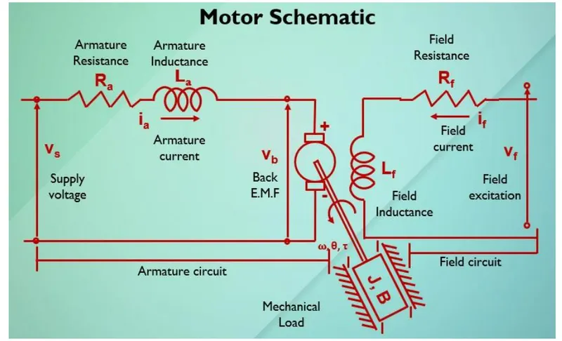
The motor torque is proportional to only the armature current by a constant Kt i.e., `T = Kt*i`

The back EMF is proportional to the angular velocity of the shaft by a constant Km i.e., `E = Km*(d theta)/dt`

Applying Kirchhoff’s voltage law and Newton’s second law to the above circuit,

`J (d^2 theta)/dt^2+B(d theta)/dt = Kt*i`

`La*(di)/dt+Ra*I = V – Km*(d theta)/dt`

The transfer function is given by,

`s(J*s+B)*theta(s) = Kt*I(s)`

`(La*s+Ra)*I(s) = V(s) – Km*s*theta(s)`

On considering the rotational speed as output and armature voltage as input,

`P(s) = (theta^.(s))/(V(s)) = (Kt)/((J*s+B)*(La*s+Ra)+(Kt-Km))`

In state space form, (`(d theta)/dt = omega`)

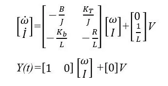
The physical parameters for our model are mentioned below,

Moment of inertia of the rotor (J) = 0.01 kg/m^2

Motor viscous friction constant (B) = 0.1 N.m.s

Back EMF constant (Km) = 0.01 V/rad/sec

Motor torque constant (Kt) = N.m/Amp

Armature resistance (Ra) = 1 Ohm

Armature Inductance (La) = 0.5 Henri

MATLAB PROGRAM:

clear all
close all
clc

% Design parameters to model a DC motar
J = 0.01; % Moment of inertia
B = 0.1; % viscous friction constant
Km = 0.01; % Back EMF constant
Kt = 0.01; % Motar torque constant
Ra = 1.0; % Resistance in ohm
La = 0.5; % Inductance in henri

% State equations
A = [-B/J Kt/J; -Km/La -Ra/La]
b = [0; 1/La]

% The transfer function is given by
s=tf('s');

Trans_fun = Kt/((J*s+B)*(La*s+Ra)+(Kt-Km))

% Placements of poles

r = roots([J*La J*Ra+B*La B*Ra+Kt*Km]); % roots command is used to find the roots of the Tf equation
P1 = r(1)
P2 = r(2)
k = place(A,b,r);
Kp = k(1)
Kd = (2)

%Stability check
pzmap(Trans_fun) % pzmap plots the poles, the poles lie on the left of the Jw plane. Hence the system is stable.
grid

The above code specifies the physical parameters also the frequency, angular velocity, and zeta are loaded. The MATLAB command 'place' is used to compute a gain matrix K such that the state feedback u = –Kx places the closed-loop poles at the locations p. The Kp and the Kd gains are obtained from the vector 'K' formed.

SIMULINK MODEL:

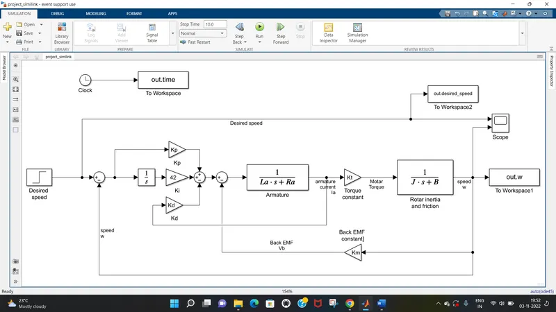
The Simulink model is built as shown below,

The output observed for speed=50,

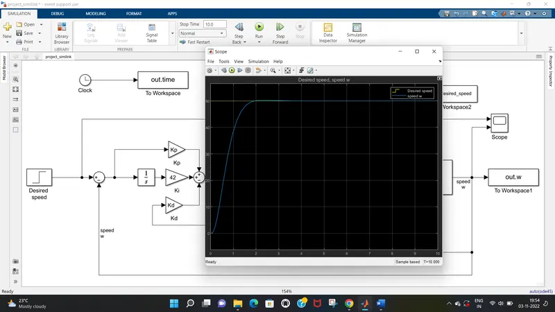
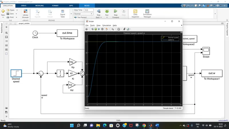
The output at speed = 100,

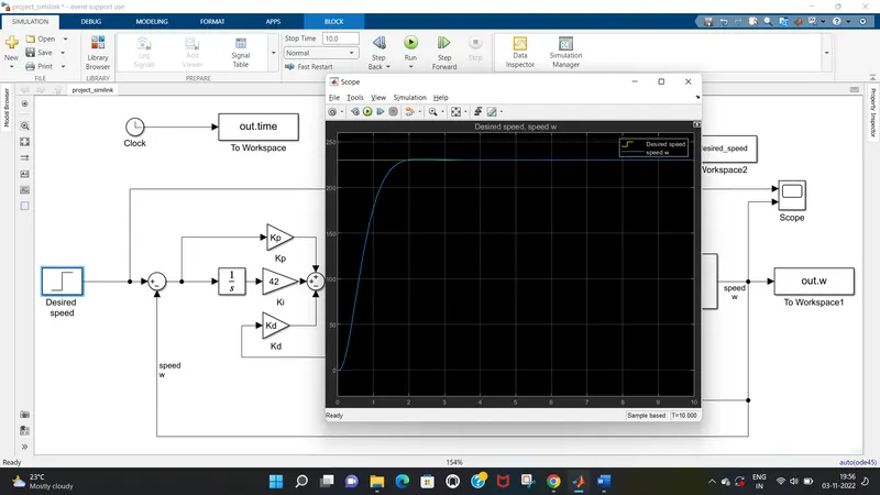
At speed = 230,

CONCLUSION:

1. The Simulink model is built for the DC motor for speed control.
2. The MATLAB code is written which intakes the parameters. And also when checked for stability it was found that the poles lie on the left side of the s plane.
3. The gain constants are determined for the Simulink model in the MATLAB script using the commands like roots and place.
4. The model was executed for various speeds such as 50, 100, and 230. It was observed that the overshoot, settling time and steady-state errors were minimal.

REFERENCE:

https://ctms.engin.umich.edu/CTMS/index.php?example=MotorSpeed&section=SystemAnalysis

https://skill-lync.com/knowledgebase/modeling-of-dc-motor