Project - Speed Control of a Direct Current (DC) motor

AIM

Speed Control of a Direct Current (DC) motor

THEORY

DC MOTOR

A DC motor is any of a class of rotary electrical motors that converts direct current (DC) electrical energy into mechanical energy. The most common types rely on the forces produced by magnetic fields. A DC motor's speed can be controlled over a wide range, using either a variable supply voltage or by changing the strength of current in its field windings. A coil of wire with a current running through it generates an electromagnetic field aligned with the center of the coil. The direction and magnitude of the magnetic field produced by the coil can be changed with the direction and magnitude of the current flowing through it.

A simple DC motor has a stationary set of magnets in the stator and an armature with one or more windings of insulated wire wrapped around a soft iron core that concentrates the magnetic field. The windings usually have multiple turns around the core, and in large motors there can be several parallel current paths. The ends of the wire winding are connected to a commutator. The commutator allows each armature coil to be energized in turn and connects the rotating coils with the external power supply through brushes.

The total amount of current sent to the coil, the coil's size, and what it is wrapped around decide the strength of the electromagnetic field created.The sequence of turning a particular coil on or off dictates what direction the effective electromagnetic fields are pointed. By turning on and off coils in sequence, a rotating magnetic field can be created. These rotating magnetic fields interact with the magnetic fields of the magnets (permanent or electromagnets) in the stationary part of the motor (stator) to create a torque on the armature which causes it to rotate. In some DC motor designs, the stator fields use electromagnets to create their magnetic fields which allows greater control over the motor.

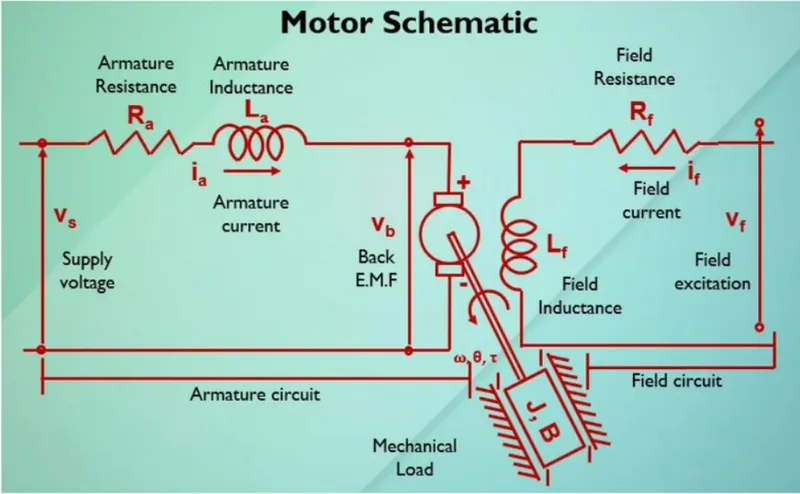
theta - position of the rotor

w(omega) - angular velocity of rotor

T(taw) - Torque of the rotor

PID CONTROLLER

A proportional–integral–derivative controller (PID controller or three-term controller) is a control loop mechanism employing feedback.A PID controller continuously calculates an error value e(t) as the difference between a desired set point (SP) and a measured process variable (PV) and applies a correction based on proportional, integral, and derivative terms (denoted P, I, and D respectively).

Mathematically the control function u(t) is given as:

DC Motor modeling

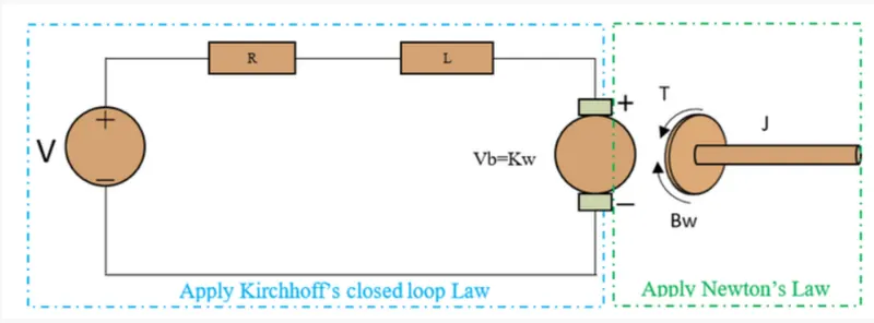
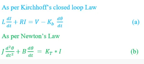
Let us assume the constants :

Motor torque T= Kt*I

Back emf Vb = Kb*w

Converting to the above equations (a) and (b) to Laplace domain:

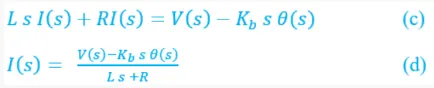
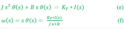
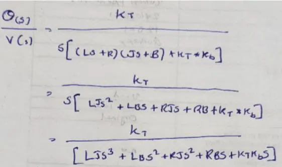
Substuting I(s) in equation (e) and simplifiying the transfer function of output angle theta(s) to input voltage V(s) is given by:

Transfer function of Position theta(s) to input voltage is given by :

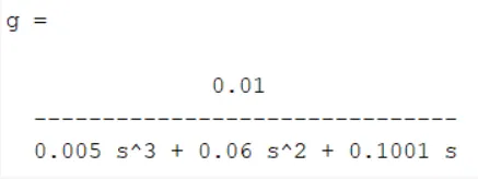
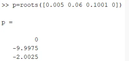
Poles of the equation is obtained using pole placement method as: p =[ 0; -9.9975; -2.0025]

Transfer function of angular velocity w(s) to input voltage V(s) is given by:

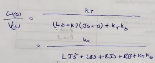
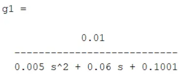
Poles of the equation is obtained by pole placement method as: p =[-9.9975; -2.0025]

State-Space Equation for DC motor

From equation (a) & (b)

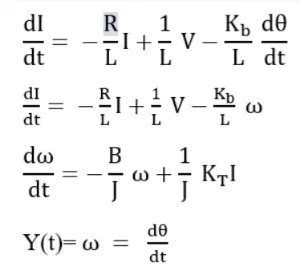
From above equation the State - Space equation can be written as:

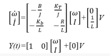
PROGRAM CODE

% DC motor speed control model
close all
clear all
clc

J=0.01; % Moment of inertia of rotor in Kg-m^2
B=0.1;  % Motor viscous friction constant n-m-s
Kb=0.01;% Back emf constant V/radian/s
Kt=0.01;% Motor torque constant N-m/A
R=1;    % Resistance of the armature circuit ohm
L=0.5;  % Inductance of armature circuit in henries

X=[-B/J Kt/J; -Kb/L -R/L];
Y=[0;1/L];
P=roots([0.005 0.06 0.1001]);

K=place(X,Y,P);

% optimum values
Kp=200;
Kd=100;
Ki=4000;

Plotting Code

%plotting
close all

subplot(321);
plot(out.time,out.vs);
title('Referecne Speed');
grid on;
subplot(322);
plot(out.time,out.w);
title('speed (w)');
grid on;
subplot(323);
plot(out.time,out.ia);
title('armature current');
grid on;
subplot(324);
plot(out.time,out.t);
title('torque');
grid on;
subplot(325);
plot(out.time,out.Vb);
title('Back emf');
grid on;
subplot(326);
plot(out.time,out.u);
title('Control - u');
grid on;

CODE EXPLAINATION

• The code begins with closeing and clearing the temperory file and memory using close all, clear all, & clc.
• Then the constants were defined.
• From the state space equation the matrix A & B were defined.Then the transfer function is made and found the poles of the transfer function using pzmap() command
• After finding the poles the K matrix has to be calculated and is done using the place() command.
• After running the matlab code and then running the sumulink model the output values will be avaliable at the workspace for plotting.
• All the previous plots if present were closed with close all command.
• Using subplot() command multiple plots were made,grid is set on using grid on,and title is given for each subplot using title() command

SIMULINK MODEL

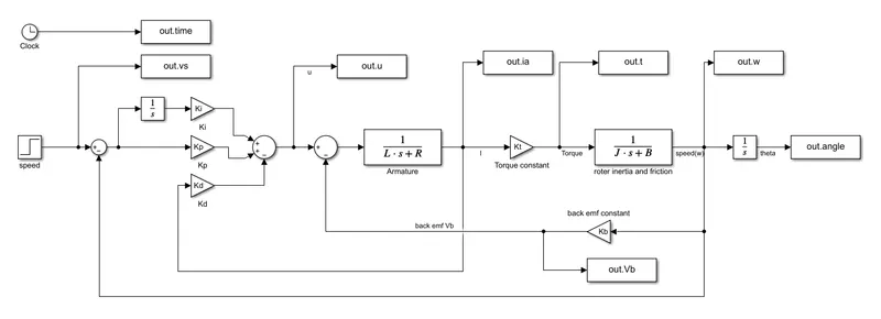
MODEL EXPLAINATION

• The reference signal is taken as a step block  from source library.
• The reference signal speed is set to 20 at time =  2 second the Block parameter.
• For summing the signals sum block from the Math operation library is used
• The gain block from math operation is used for multiplying the signals.
• The reference signal is integrated once to get the position using the integrator block obtained from continuous library.
• The initial position of intergrator block is set to 0.01.
• To workspace block from sink library is used to display the signals.
• The poles of the transfer function are obtained by using the transfer function and roots() command 
• Then by getting the value of A B & P the values of K matrix is obtained using place() command.This will give the values of Kp & Kd.

OUTPUT

Before tunning Kp, Kd & Ki (Kp & Kd from pole placement Ki=0)

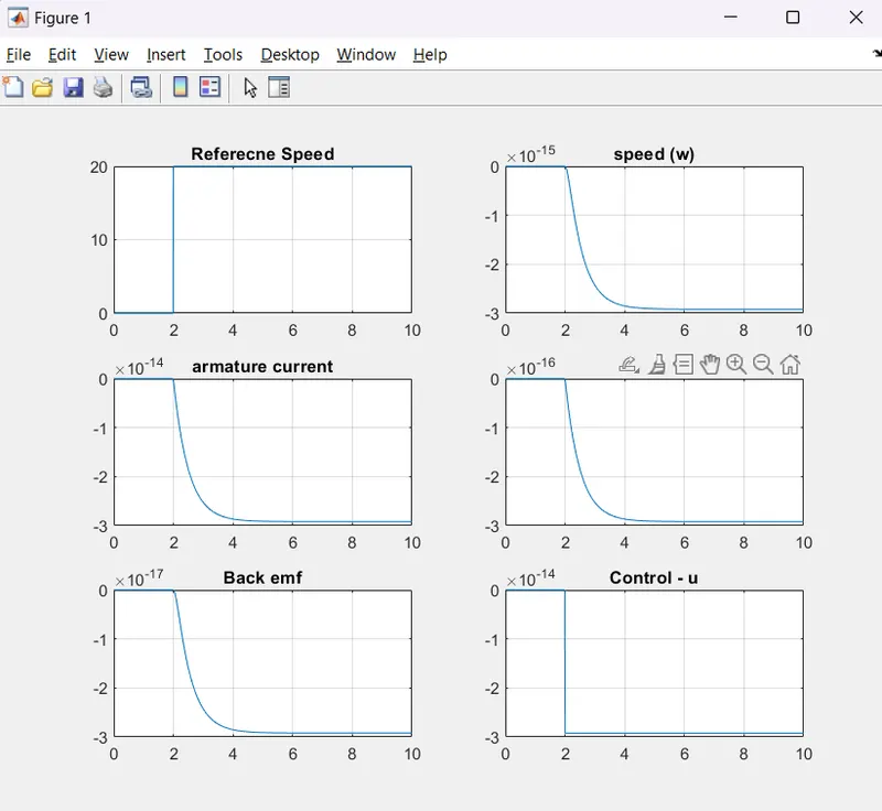
The speed output is not at all near the reference speed.so Ki has to be introduced and tuned.

After Tunning Ki = 4000 Keeping Kp & Kd same

 

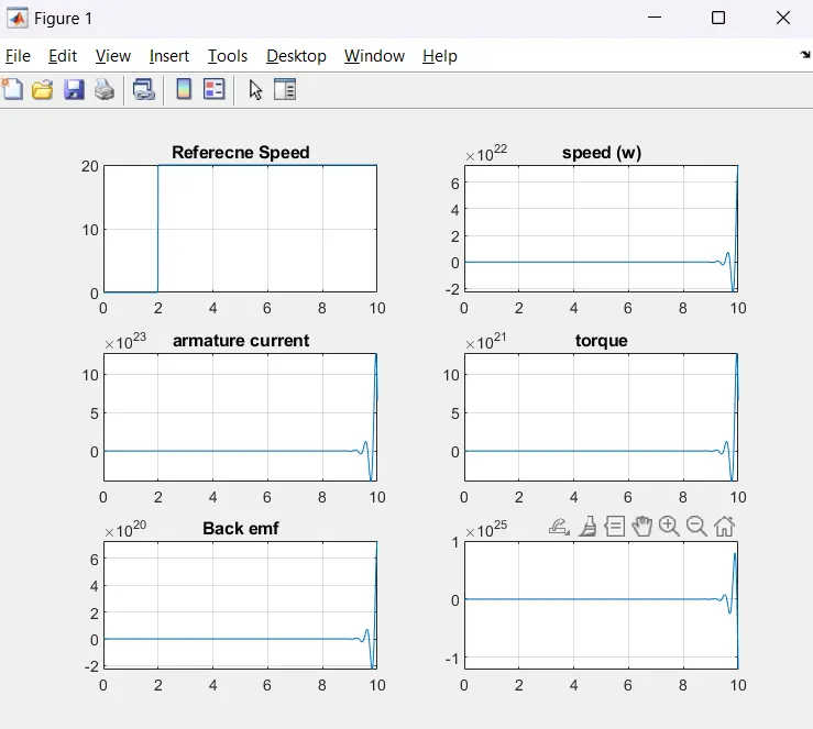
When Ki is intorduced the speed value shoots above the required speed with osillation,but when compared to the model without Ki the signal is responding better.

After Tunning Kp=100 Ki= 4000 & Kd same

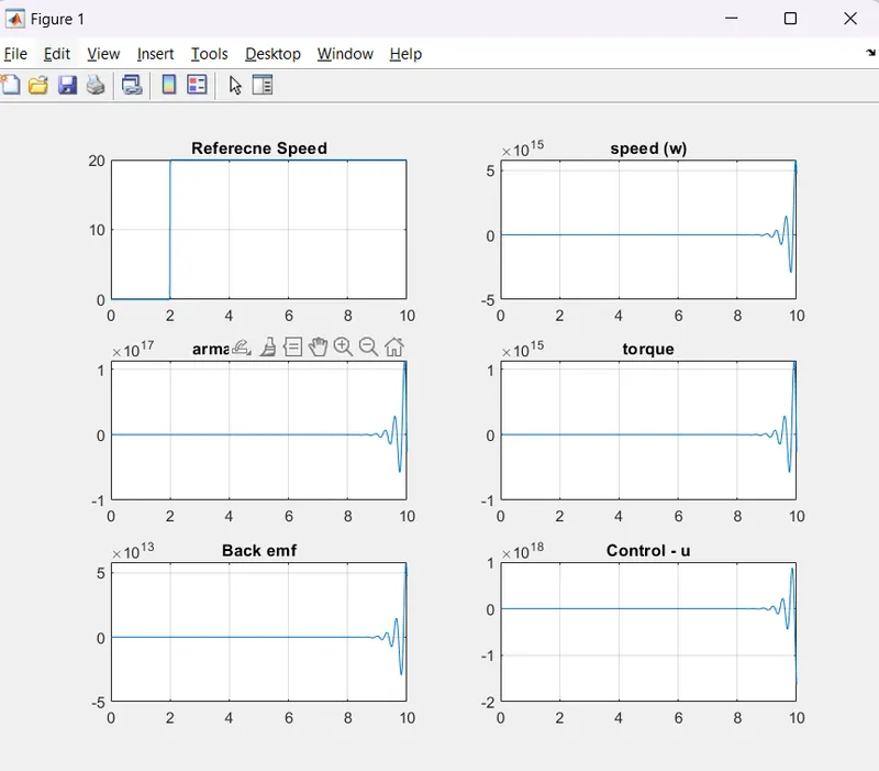
With these values of Kp Ki & Kd the speed out was found to be decreasing from what we saw in previous graph , which means the output is comming closer to reference speed.

After Tunning Kp=100 Ki= 4000 & Kd = 100

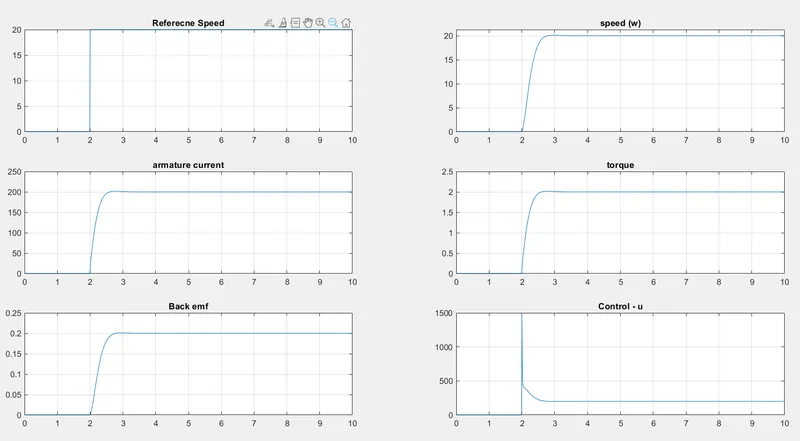
• After tunning the Kp,Kd & Ki the required output was obtained.
• Within 2 second (time=4 sec) the system came to the requires reference speed with little bit of overshoot.

After Tunning Kp, Kd & Ki 

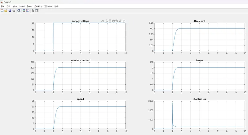
After Tunning Kp=100 Ki= 4500 & Kd = 100

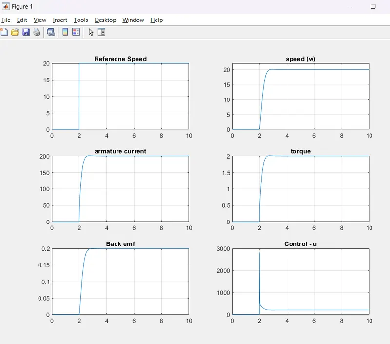
Enlarged view:

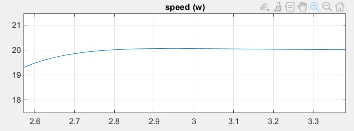
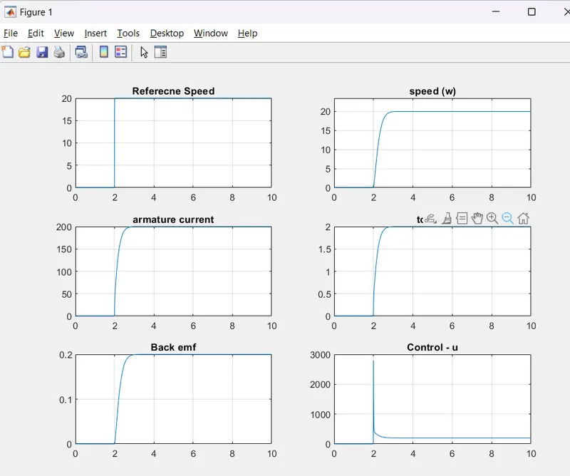
It is found that the speed settles within time = 3.3 with very little overshoot and under shoot.

After Tunning Kp=100 Ki= 4000 & Kd = 100

Enlarged  view of speed

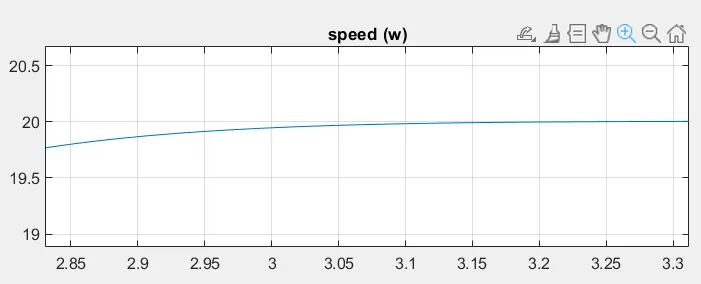
• It is found that tunning the Kp=100 Ki= 4000 & Kd = 100 gives the perfect optimal values for the design.
• The system is stable and the output speed became same as reference speed of 20 rad/sec within 3.2 seconds without any overshooting or undershooting.

WORKSPACE

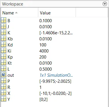
CONCLUSION

• After modeling and tunning the values of Kp, Kd & Ki the desiered output was observer without an overshoot or undershoot as well as the settling time was minimized, and also the raise time was quick.
• The step input was stated at 2 second and got stablised at speed of  20 within 3.2 second.
• The optimum values of Kp=200 Kd = 100 and Ki =4000
• Increasing the vlues beyond this leads to system failure that effecting the stability.