Project - Position control of mass spring damper system

Aim

Obtain the transfer function of a mass spring damper system and use it in the model. Add a PID controller to adjust the force on mass so that its position follows a reference signal.

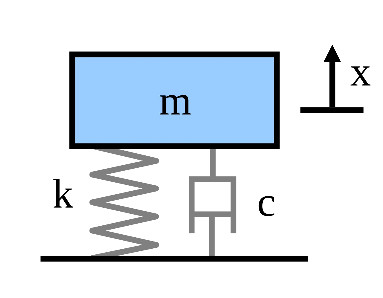
Spring mass damper system

The mass-spring-damper model consists of discrete mass nodes distributed throughout an object and interconnected via a network of springs and dampers. This model is well-suited for modelling object with complex material properties such as nonlinearity and viscoelasticity. Packages such as MATLAB may be used to run simulations of such models. As well as engineering simulation, these systems have applications in computer graphics and computer animation.

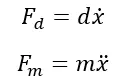
To analyze the mass-spring-damper system it is a prerequisite to understanding how to model the equations of each component with the knowledge of Newton’s 2^nd law of motion. Which are represented below.

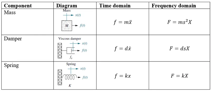
With the following points of consideration, the modelling is done.

• Point masses are present only
• is resultant of all forces
• is absolute acceleration
• Linear force in direction is acting.

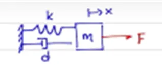
The following free body diagram (FBD) in a positive deflected state is presented.

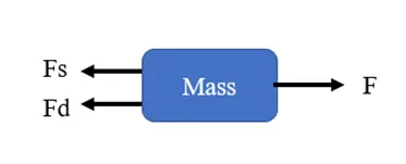
The sum of all forces acting in a different direction is given as follows,

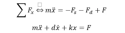
This is the equation of motion (EoM) and it is in the form of 2^nd order ordinary differential equation (ODE), linear in nature, with constant coefficients and inhomogeneous.

The above equation was in the differential form we can convert it into the s domain or frequency domain which is represented as follows,

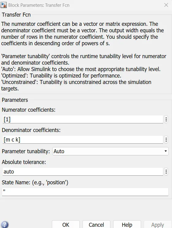
Finally, we can rearrange the equation to get the transfer function G(s) of this system. The definition of the transfer function of a control system is its outputs divided by its inputs. In this case, X(s) is the output, F(s) is the input, so we can get G(s) as follows:

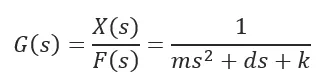
The above-derived ODE can be converted to a single order equation by using a state-space representation of the mass-spring damper system. The Laplace transformation ignores the initial condition of the system.

PID controller

A proportional–integral–derivative controller (PID controller or three-term controller) is a control loop mechanism employing feedback that is widely used in industrial control systems and a variety of other applications requiring continuously modulated control. A PID controller continuously calculates an error value as the difference between a desired setpoint (SP) and a measured process variable (PV) and applies a correction based on proportional, integral, and derivative terms (denoted P, I, and D respectively), hence the name.

In practical terms, PID automatically applies an accurate and responsive correction to a control function. An everyday example is the cruise control on a car, where ascending a hill would lower speed if constant engine power were applied. The controller's PID algorithm restores the measured speed to the desired speed with minimal delay and overshoot by increasing the power output of the engine in a controlled manner.

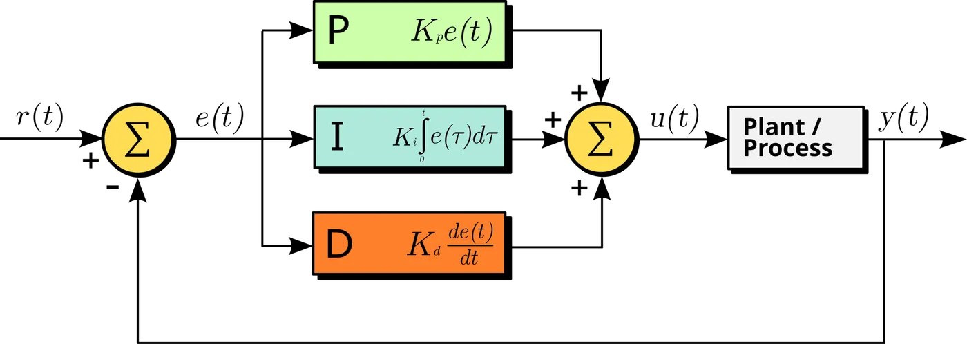
The overall control function �(�)=�p�(�)+�i∫0��(�)d�+�dd�(�)d�,

where �p, �i, and �d, all non-negative, denote the coefficients for the proportional, integral, and derivative terms respectively (sometimes denoted P, I, and D).

Implementation of Spring mass system using PID controllers

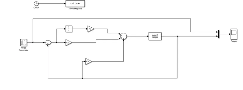
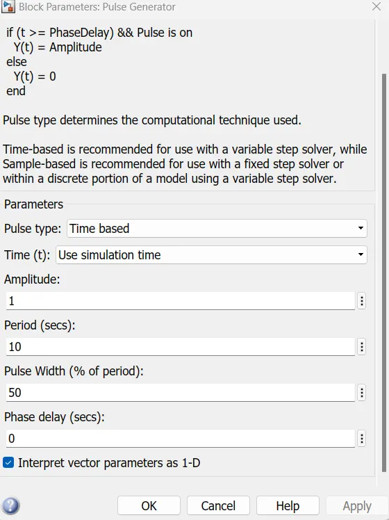
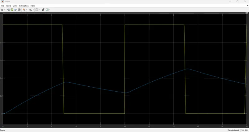
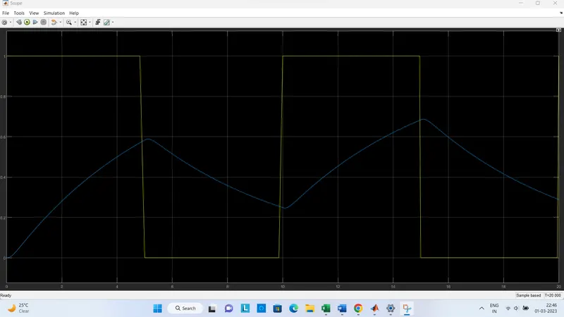
The Simulink model of Spring mass damper system along with PID controller is shown below

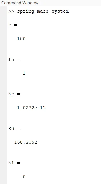
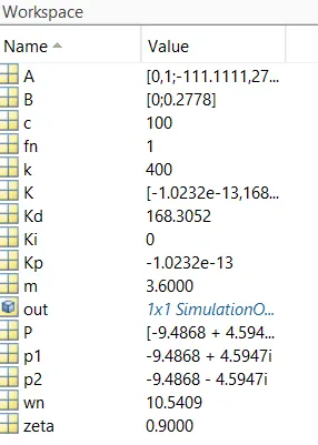
Intial conditions are defined below

m=3.6; %Mass of the spring

k =400 ; %Spring constant

c=100 %Damping coefficient

fn=1.0 % Natural frequency in Hz

wn = sqrt(k/m) ; % Natural frequency in rad/sec

zeta=0.9; % Underdamped behaviour

p1= -zeta*wn+wn*sqrt(zeta^2-1);

p2=-zeta*wn-wn*sqrt(zeta^2-1);

P=[p1;p2];

A=[ 0 1 ; -k/m c/m];

B=[0 ; 1/m];

%Pole placement design

K=place(A,B,P);

Kp= K(1)

Kd=K(2)

Ki=0

Intially Ki was set to zero

Running the above conditions in matlab and updating the Kp , Ki and Kd gains in Simulink model and running the model

Workspace results:

Output results:

Explanation:

1 . The input refrence signal is inputed through the system by using Pulse generator having amplitude of 1 and period of 10 seconds as shown in figure below

2 The transfer function of Spring mass damper system is implemented in the system by using Transfer function

3 The input for the the Integral gain Ki is fed thorugh integrator block and refrence signal output . Intial reaponse of the Ki was set to zero to record the response with refrence signal

4 The PID gains such as Kp and Kd values are calculated by running matlab file and subsequently updated those values in the system

5 By running place command placement of pole is calculated

6 If we used the derivative block with the proportional gain to compare the output results . As we got steady state error which was overlapping overshoot response .

7 To compensate the above error we have introduced demux block to output separate signals coming from Kp and Ki gains.

Now Changing the Ki values and outputing results through scope block

Setting Ki as 50

As we can see from the above plot we can observe that rise time and settling time is decreasing

Increasing Ki value to 100

The output signal is not following refrence signal

Increasing the value of Ki to 600

From the above plot we can clearly observe that the output follows refrence signal

Conclusion

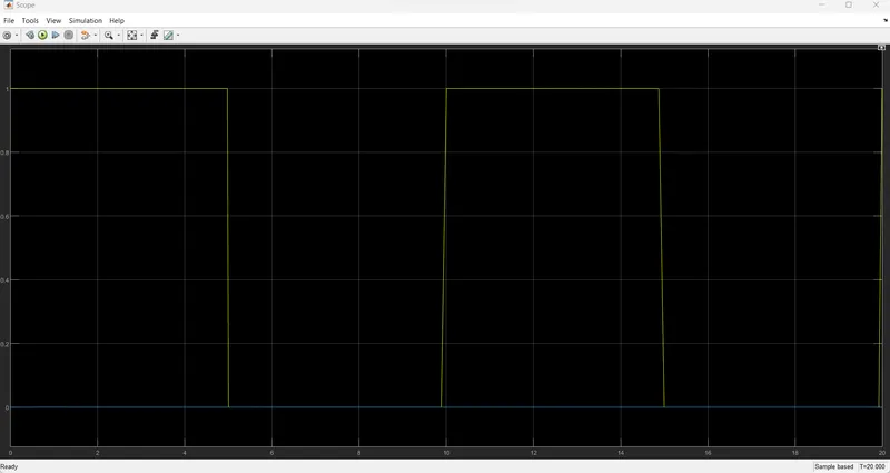
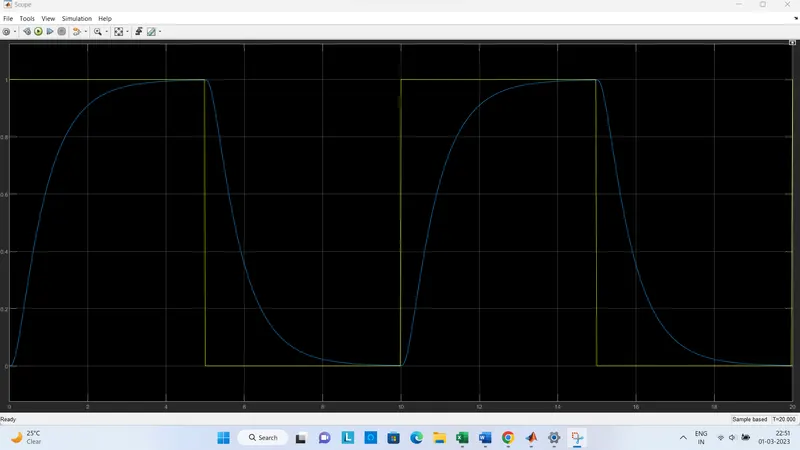
With the help of PID controllers we have successfully positioned the spring mass damper system.