Project 1 - Parsing NASA thermodynamic data

Aim

To write MATLAB code to extract data from NASA thermodynamic data file

Objective

1 Calculating molecular weight of each species

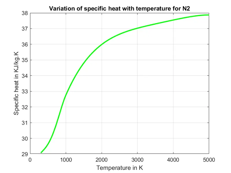
2 Plotting Enthalpy , Entropy and specific heat of various species with refrence to variation in temperature.

Introduction

This deals with the filed of computational linguistics where it commonly defines Natural language processing

Natural lanuage processing (NLP) , is concerned with programming with computers to process and analyse the human written language .

Parser helps to split the large input data into smaller data and will process the data .

Parsing is necessary because different application needs data to be present in different forms . Parsing allows transforming that data in a way that can be understood by specific software . The obvious example is programs- that is written by humans , but they must be executed by computers .

Parsing helps to automate certain things , and also reduces human effort .

And can be used for applications like Machine learing , automation etc.

Understanding NASA Thermodynamic Data file

The File includes the NASA Thermodynamic data file . Having total of 53 Species with three local temperatures and 14 coefficinets in total of each species .

The coefficients of two catagories , such as high temperature coefficients (first 7 coefficients ) and low temperature coefficients (second 7 coefficients)

Molecular weight of each species is calculated.

After calculating specific heat, enthalpy and entropy, variation of it is plotted with respect to temperature for each species.

Following mathematical relations are used to calculate specific heat, enthalpy, and entropy, respectively.

Where Cp is specific heat at constant pressure, R is universal gas constant, H is enthalpy, S is entropy and T is temperature.

Reading the file

The file should be loaded and opened in the script using the ‘fopen’

And The lines necessary for the calculation should be get from the file using ‘fgetl’

Parsing Species block

The first seven coefficients are hight temperature coefficients and second seven denotes the low temperature coefficients

Code explanation

1. Given .dat file is read by using ‘fopen(' THERMO.dat', 'r')

   f1 = fopen('THERMO.dat', 'r');​

2. By using ‘fget(l)’ command, first line (THERMO)is read.

   fgetl(f1);​

3. Global temperatures (2^nd line of file) is read by using ‘aa = fgetl(f1)’. Then this line is spitted by using ‘fget(l)’ command. Then global temperatures (300, 1000 and 5000) are read.

   aa = fgetl(f1);
   tt = strsplit(aa, ' ');
   global_low_temp = str2num(tt{2});
   global_mid_temp = str2num(tt{3});
   global_high_temp = str2num(tt{4});
   

4. Line no 3, 4 and 5 are read using ‘fget(l)’ command.

    To eliminate comment lines
   for i=3:5
        fgetl(f1);
   end​

5. Now each species has 4 lines. First line contains the species name and local temperatures (low, middle and high temperature). Next line

   (O L 1/90O 1 G 200.000 3500.000 1000.000 1)

   is read by using ‘fget(l)’ command. Then to identify the species, above line is splitted using ‘fget(l)’ command and name species is identified.

   for j=1:53
   tline=fgetl(f1);
   A = strsplit(tline, ' ');
   species = (A{1});​

6. Now to determine the values of low, middle, and high temperature, the location of dot(.) is identified and with respect to position of dot(.) values of low, middle, and high temperature are read.

   pos_dot=strfind(tline,'.');
   low_temp = tline(pos_dot(1)-3:pos_dot(1)+3);
   low_temp = str2num(low_temp);
   high_temp = tline(pos_dot(2)-4:pos_dot(2)+3);
   high_temp =  str2num(high_temp);
   mid_temp = tline(pos_dot(3)-4:pos_dot(3)+3);
   mid_temp =  str2num(mid_temp);​

7. Similarly, next 3 lines are read using ‘fget(l)’ command. First and second line has 5 coefficients each and 3^rd line has 4 coefficients. To read value of each coefficient, position of ‘E’ has been found out in each line and with respect to position of ‘E’ each coefficient value is read.

   dataline_1 = fgetl(f1);
   dataline_2 = fgetl(f1);
   dataline_3 = fgetl(f1);
   
   A = strfind(dataline_1,'E');
   B = strfind(dataline_2,'E');
   C = strfind(dataline_3,'E');​

8. Temperature values are specified using ‘linspace’ command and value of R is defined.

   T = linspace(low_temp, high_temp,500);
   R = 8.314;

   1. Specific heat, enthalpy and Entropy is calculated.

9. for i=1:length(T)
       if T(i)>mid_temp
           cp(i)= (t1+t2.*T(i)+t3.*T(i).^2+t4.*T(i).^3+t5.*T(i).^4)*R;
           H(i)= R*T(i).*(t1+((t2*T(i)/2))+((t3*T(i).^2)/3)+((t4*T(i).^3)/4)+((t5*T(i).^4)/5)+((t6./T(i))));
           S(i)= (t1.*log(T(i))+t2.*T(i)+t3.*(T(i)^2)/2+t4.*(T(i)^3)/3+t5.*(T(i)^4)/4+t7)*R;
       else
           cp(i)= (t8+t9.*T(i)+t10.*T(i).^2+t11.*T(i).^3+t12.*T(i).^4)*R;
           H(i)= R*T(i).*(t8+((t9*T(i)/2))+((t10*T(i).^2)/3)+((t11*T(i).^3)/4)+((t12*T(i).^4)/5)+((t13./T(i))));
           S(i)= (t8.*log(T(i))+t9.*T(i)+t10.*(T(i)^2)/2+t11.*(T(i)^3)/3+t12.*(T(i)^4)/4+t14)*R;
       end
   end

10. hen variation of specific heat, enthalpy and entropy are plotted with respect to temperature.

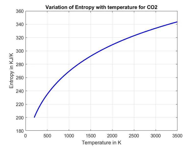
    % To plot varation of cp with T
    figure(1)
    plot(T, cp, 'linewidth',2,'color','g')
    xlabel('Temperature in K')
    ylabel('Specific heat in KJ/kg.K')
    grid on
    title(sprintf('Variation of specific heat with temperature for %s', species))
    saveas(figure(1),'cp.png');
    
    % To plot variation of enthapy with temperarure
    figure(2)
    plot(T, H, 'linewidth',2,'color','r')
    xlabel('Temperature in K')
    ylabel('Enthalpy in KJ/kg')
    grid on
    title(sprintf('Variation of Enthalpy with temperature for %s', species))
    saveas(figure(2),'H.png');
    
    % To plot variation of entropy with temperarure
    figure(3)
    plot(T, S, 'linewidth',2,'color','b')
    xlabel('Temperature in K')
    ylabel('Entropy in KJ/K')
    grid on
    title(sprintf('Variation of Entropy with temperature for %s', species))
    saveas(figure(3),'S.png');​

11. Molecular weight is calculated.

    % To calculate molecular weight
     Molecular_wt = molecular_weight(species);
     k = sprintf('Molecular weight of %s is %f', species,Molecular_wt);
     disp(k)​

12. One folder is created named ‘species’ and all plots are saved in that folder, species wise separately.
    cd('C:\Users\vishn\OneDrive\Documents\MATLAB\Parsing')

    mkdir(species);

    cd(species);

    Function code to calculate Molecular weight

    function[molecular_weight] = molecular_weight(species)
    elements = {'H','C','O','N','A','S'};
    atomic_weight = [1,12,16,14,39,32];
    molecular_weight=0;
     for i=1:length(species)
         for j=1:length(elements)
             if strcmp(species(i),elements(j))
                 molecular_weight = molecular_weight+atomic_weight(j) 
                 a=j;
             end
             end  
           n = str2num(species(i));
           if(n>1)
                 molecular_weight = molecular_weight+(atomic_weight(a)*(n-1))
         end
     end
    end

    Complete code

13. clear all
    close all
    clc
    % Getting data from provided file
    f1 = fopen('THERMO.dat', 'r');
    fgetl(f1);
    aa = fgetl(f1);
    tt = strsplit(aa, ' ');
    global_low_temp = str2num(tt{2});
    global_mid_temp = str2num(tt{3});
    global_high_temp = str2num(tt{4});
    % To eliminate comment lines
    for i=3:5
    fgets(f1)
    end
    % To get species data
    for j=1:53
    tline=fgetl(f1);
    A = strsplit(tline, ' ');
    species = (A{1});
    pos_dot=strfind(tline,'.');
    low_temp = tline(pos_dot(1)-3:pos_dot(1)+3);
    low_temp = str2num(low_temp);
    high_temp = tline(pos_dot(2)-4:pos_dot(2)+3);
    high_temp = str2num(high_temp);
    mid_temp = tline(pos_dot(3)-4:pos_dot(3)+3);
    mid_temp = str2num(mid_temp);
     
    dataline_1 = fgetl(f1);
    dataline_2 = fgetl(f1);
    dataline_3 = fgetl(f1);
    A = strfind(dataline_1,'E');
    B = strfind(dataline_2,'E');
    C = strfind(dataline_3,'E');
    t1 = dataline_1(1:A(1)+3);
    t1 = str2num(t1);
    t2 = dataline_1(A(1)+4:A(2)+3);
    t2 = str2num(t2);
    t3 = dataline_1(A(2)+4:A(3)+3);
    t3 = str2num(t3);
    t4 = dataline_1(A(3)+4:A(4)+3);
    t4 = str2num(t4);
    t5 = dataline_1(A(4)+4:A(5)+3);
    t5 = str2num(t5);
    t6 = dataline_2(1:B(1)+3);
    t6 = str2num(t6);
    t7 = dataline_2(B(1)+4:B(2)+3);
    t7 = str2num(t7);
    t8 = dataline_2(B(2)+4:B(3)+3);
    t8 = str2num(t8);
    t9 = dataline_2(B(3)+4:B(4)+3);
    t9 = str2num(t9);
    t10 = dataline_2(B(4)+4:B(5)+3);
    t10 = str2num(t10);
    t11 = dataline_3(1:C(1)+3);
    t11 = str2num(t11);
    t12 = dataline_3(C(1)+4:C(2)+3);
    t12 = str2num(t12);
    t13 = dataline_3(C(2)+4:C(3)+3);
    t13 = str2num(t13);
    t14 = dataline_3(C(3)+4:C(4)+3);
    t14 = str2num(t14);
    T = linspace(low_temp, high_temp,500);
    R = 8.314;
    % specific heat, Entahlpy and Entropy calculation
    for i=1:length(T)
    if T(i)>mid_temp
    cp(i)= (t1+t2.*T(i)+t3.*T(i).^2+t4.*T(i).^3+t5.*T(i).^4)*R;
    H(i)= R*T(i).*(t1+((t2*T(i)/2))+((t3*T(i).^2)/3)+((t4*T(i).^3)/4)+((t5*T(i).^4)/5)+((t6./T(i))));
    S(i)= (t1.*log(T(i))+t2.*T(i)+t3.*(T(i)^2)/2+t4.*(T(i)^3)/3+t5.*(T(i)^4)/4+t7)*R;
    else
    cp(i)= (t8+t9.*T(i)+t10.*T(i).^2+t11.*T(i).^3+t12.*T(i).^4)*R;
    H(i)= R*T(i).*(t8+((t9*T(i)/2))+((t10*T(i).^2)/3)+((t11*T(i).^3)/4)+((t12*T(i).^4)/5)+((t13./T(i))));
    S(i)= (t8.*log(T(i))+t9.*T(i)+t10.*(T(i)^2)/2+t11.*(T(i)^3)/3+t12.*(T(i)^4)/4+t14)*R;
    end
    end
    % Saving in a folder
    cd('C:\Users\vishn\OneDrive\Documents\MATLAB\Parsing')
    mkdir(species);
    cd(species);
    % To plot varation of cp with T
    figure(1)
    plot(T, cp, 'linewidth',2,'color','g')
    xlabel('Temperature in K')
    ylabel('Specific heat in KJ/kg.K')
    grid on
    title(sprintf('Variation of specific heat with temperature for %s', species))
    saveas(figure(1),'cp.png');
    % To plot variation of enthapy with temperarure
    figure(2)
    plot(T, H, 'linewidth',2,'color','r')
    xlabel('Temperature in K')
    ylabel('Enthalpy in KJ/kg')
    grid on
    title(sprintf('Variation of Enthalpy with temperature for %s', species))
    saveas(figure(2),'H.png');
    % To plot variation of entropy with temperarure
    figure(3)
    plot(T, S, 'linewidth',2,'color','b')
    xlabel('Temperature in K')
    ylabel('Entropy in KJ/K')
    grid on
    title(sprintf('Variation of Entropy with temperature for %s', species))
    saveas(figure(3),'S.png');
     
    cd('C:\Users\vishn\OneDrive\Documents\MATLAB\Parsing')
     
    % To calculate molecular weight
    Molecular_wt = molecular_weight(species);
    k = sprintf('Molecular weight of %s is %f', species,Molecular_wt);
    disp(k)
    end
    

14. Coefficients

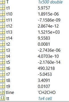
    >> t1

    t1 =

    5.9757

    >> t2

    t2 =

    0.0081

    >> t3

    t3 =

    -2.7436e-06

    >> t4

    t4 =

    4.0703e-10

    >> t5

    t5 =

    -2.1760e-14

    >> t6

    t6 =

    490.3218

    >> t7

    t7 =

    -5.0453

    >> t8

    t8 =

    3.4091

    >> t9

    t9 =

    0.0107

    >> t10

    t10 =

    1.8915e-06

    >> t11

    t11 =

    -7.1586e-09

    >> t12

    t12 =

    2.8674e-12

    >> t13

    t13 =

    1.5215e+03

    >> t14

    t14 =

    9.5583

    >>

15. Screenshot of the window where all the folders are saved.

Plot for o2

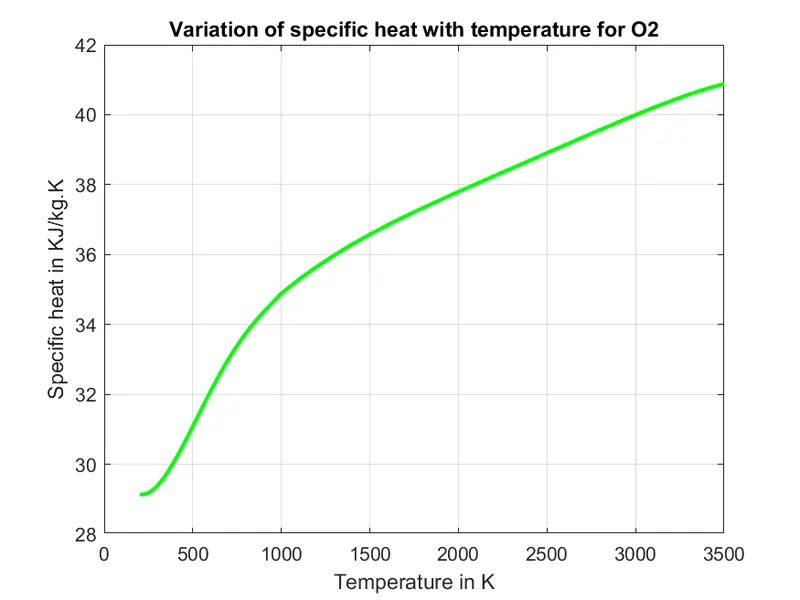
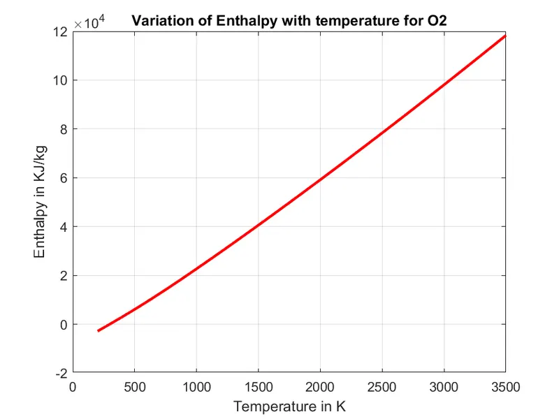
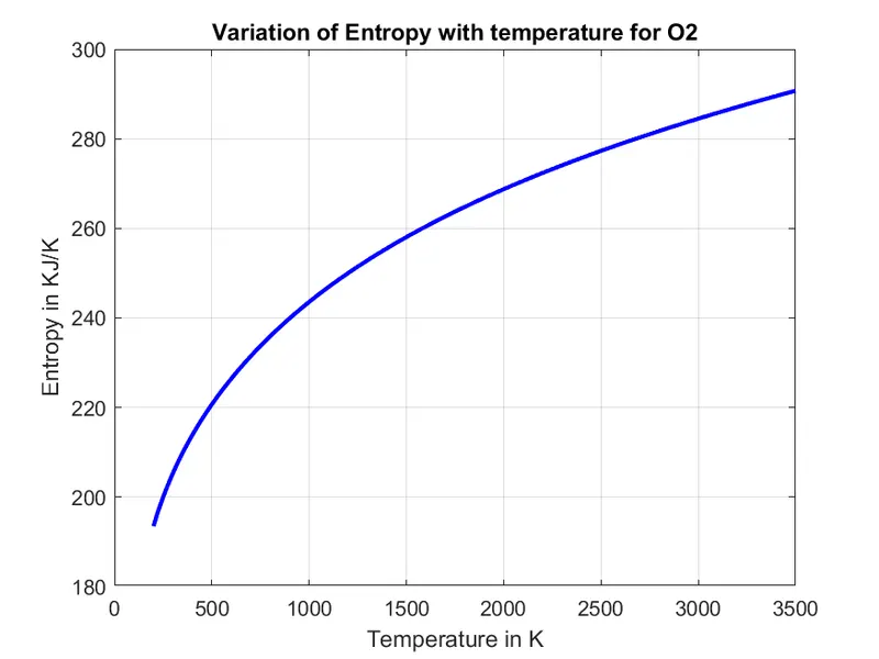
Plot for N2

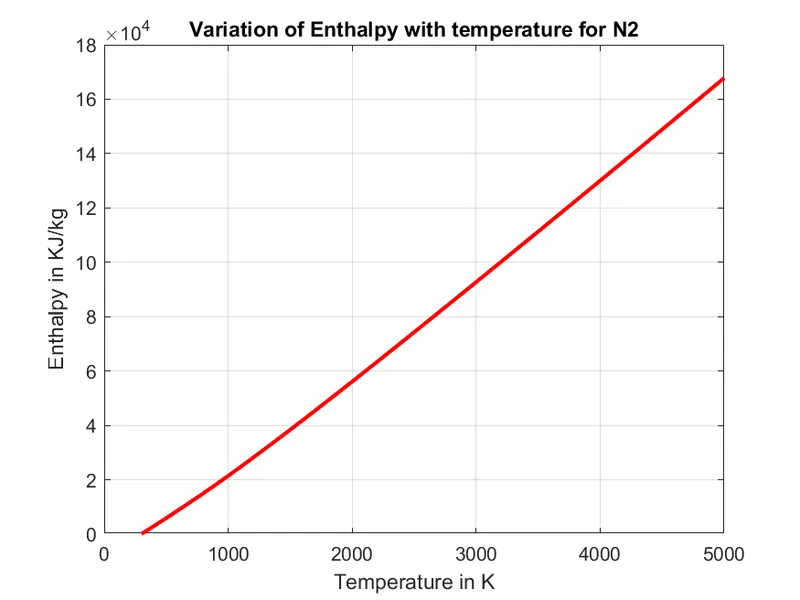
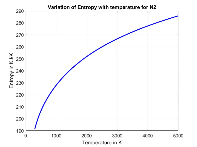
Plot for Co2

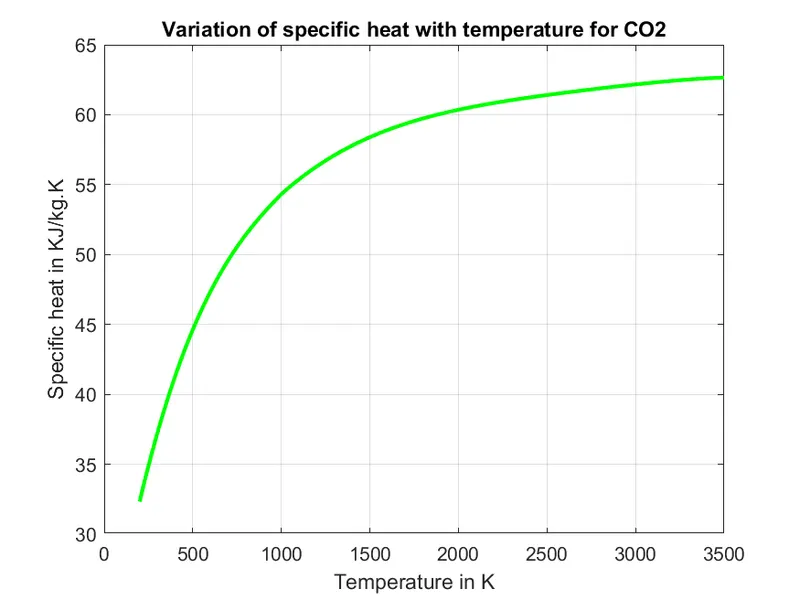
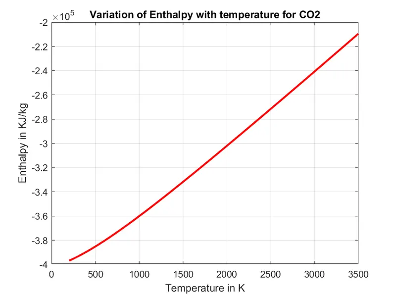
The plots for remaining species can be acessed by google drive link below

https://drive.google.com/drive/folders/135qnozyokpp836kVpg--XcjxHEgDnwcC?usp=sharing

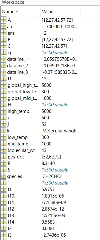
workspace

Conclusion

Extracted NASA Thermodynamic data file using File parsing

Calculated the molecular weight of each species and plots for Enthalpy , Entropy and specific heat of various species with refrence to variation in temperatur are obtained .