Week 5 - Genetic Algorithm

Aim

To optimise the stalagmite function and find the global maxima of the function.

Objective

Explaining the concept of genetic algorithm and syntax for ga in Matlab

Plot graphs for all 3 iterations and F maximum vs no. of iterations

Genetic algorithm

The genetic algorithm is a method for solving both constrained and unconstrained optimization problems that is based on natural selection, the process that drives biological evolution. The genetic algorithm repeatedly modifies a population of individual solutions. At each step, the genetic algorithm selects individuals from the current population to be parents and uses them to produce the children for the next generation. Over successive generations, the population "evolves" toward an optimal solution. You can apply the genetic algorithm to solve a variety of optimization problems that are not well suited for standard optimization algorithms, including problems in which the objective function is discontinuous, nondifferentiable, stochastic, or highly nonlinear. The genetic algorithm can address problems of mixed integer programming, where some components are restricted to be integer-valued.

Process flow

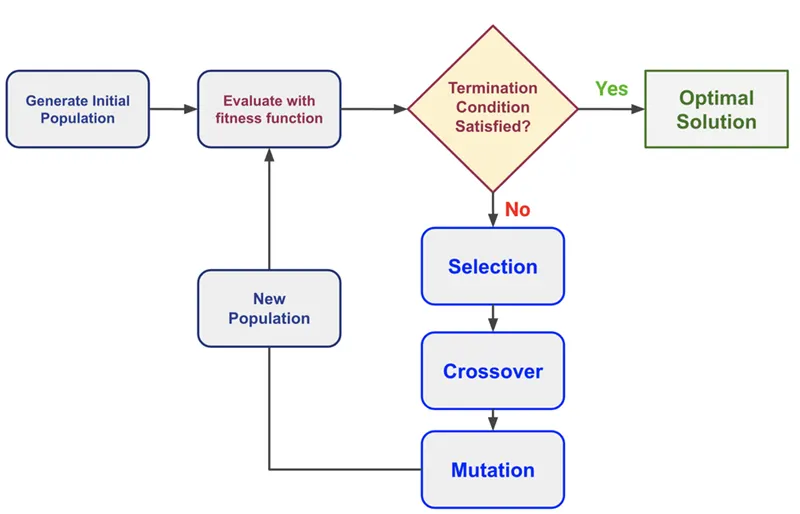
Outline of the Algorithm

The following outline summarizes how the genetic algorithm works:

1. The algorithm begins by creating a random initial population.
2. The algorithm then creates a sequence of new populations. At each step, the algorithm uses the individuals in the current generation to create the next population. To create the new population, the algorithm performs the following steps:
   1. Scores each member of the current population by computing its fitness value. These values are called the raw fitness scores.
   2. Scales the raw fitness scores to convert them into a more usable range of values. These scaled values are called expectation values.
   3. Selects members, called parents, based on their expectation.
   4. Some of the individuals in the current population that have lower fitness are chosen as elite. These elite individuals are passed to the next population.
   5. Produces children from the parents. Children are produced either by making random changes to a single parent—mutation—or by combining the vector entries of a pair of parents—crossover.
   6. Replaces the current population with the children to form the next generation.
3. The algorithm stops when one of the stopping criteria is met.
4. The algorithm takes modified steps for linear and integer constraints.

Initial Population

The algorithm begins by creating a random initial population, as shown in the following figure

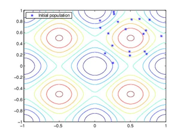
In this example, the initial population contains 20 individuals. Note that all the individuals in the initial population lie in the upper-right quadrant of the picture, that is, their coordinates lie between 0 and 1. For this example, the InitialPopulationRange option is [0;1].

If you know approximately where the minimal point for a function lies, you should set InitialPopulationRange so that the point lies near the middle of that range. For example, if you believe that the minimal point for Rastrigin's function is near the point [0 0], you could set InitialPopulationRange to be [-1;1]. However, as this example shows, the genetic algorithm can find the minimum even with a less than optimal choice for InitialPopulationRange.

Creating the Next generation

At each step , the genetic algorithm uses the current population to create the children that makes up the the next generation.

The algorithm selects a group of individuals in the current population as parents.

The algorithm usually selects individuals that have better fitness values as parents.

Selection

It defined the selection of parents for the next generation using selection function/fitness function which will be based on fitness value

Cross over

Cross over enables the algorithm to extract the best characters from different individuals and recombine them into potentially superior children

Mutation

Mutation adds to the diversity of a population and thereby increases the likelihood that the algorithm will generate individuals with better fitness values.

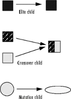
Types of children produced for next generation from the current population as follows

• Elite child: Individuals having best fitness values
• Cross over child: Created by combining the parents
• Mutation child: Created by doing random changes to single point

Stopping criteria

Max generations : The algorithm stops when the number of generations reaches Maximum generations

MaxTime : The algorithm stops after running for an amount of time in seconds equal to MaxTime.

Fitness limit : The algorithm stops when the value of fitness function for the best function for the best point in the current population is less than or equal to Fitness limit.

Syntax for Genetic algorithm (GA)

x = ga(fun,nvars,A,b,Aeq,beq,lb,ub,nonlcon,options)

fun = objective function

nvar = number of Variables (specified as an positive integer)

A,b = Linear inequality constraints(A = Real matrix , b= Real vector)

Aeq, Beq = Linear equality constraints (A=Real matrix , B=Real vector)

lb,ub= Lower bounds and upper bounds

nonlcon = Non linear constraints

options = Optimization options

Stalagmite function

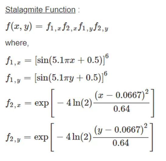
Function program:

function [f]=stalagmite(input_vector)

a=input_vector(1);
b=input_vector(2);

f1_x=[sin((5.1*pi*a)+0.5)].^6;
f1_y=[sin((5.1*pi*b)+0.5)].^6;
f2_x=exp(-4*log(2)*(((a-0.0667)^2)/(0.64)));
f2_y=exp(-4*log(2)*(((b-0.0667)^2)/(0.64)));

f=-(f1_x*f1_y*f2_x*f2_y);

end

Note : While using the function at the end as we are using the -ve sign so that the plot will be reversed as we have to find the maxima of the given function using ga.

clear
close all
clc

%% PROVIDING THE SEARCH SPACE FOR THE FUNCTION

    x=linspace(0,0.6,150);
    y=linspace(0,0.6,150);
    [X,Y]=meshgrid(x,y);
    
    num_cases=50;       %Number of itreation for which the function will evaluate the fitness


%% CREATING THE SURFACE PLOT OF STALAGEMITE FUNCTION

     for i=1:length(X)
         for j=1:length(Y)
             input_vector(1)=X(i,j);
             input_vector(2)=Y(i,j);
             f(i,j)=stalagmite(input_vector);  %values of function in given search space
         end
     end
 
        surfc(X,Y,-f);       %generating the surface
        shading interp      %To remove the lines produced by the mesh grid
 
        [inputs,fval]=ga(@stalagmite,2)

        xlabel('X axis')
        ylabel('y axis')
        title('stalagmite function')

Output of the plot

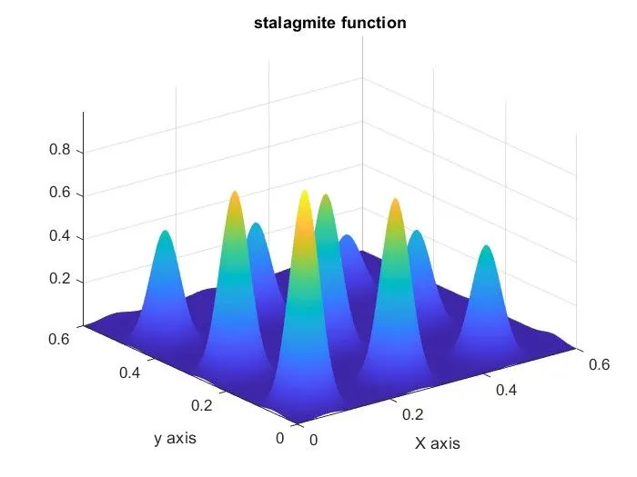
Output results:

inputs =

0.2720 0.0764

fval =

-0.7281

Code explanation :

1 Give the possible range range for ga solver

2 This inputs will be considered as space for the algorithm to solve

3 It should be practical range suitable for the problem

4 Using stalagmite function to create contour of peaks for the defined input variables with suitable range

5 It is one of the test functions used to vaildate the performance characteristics of optimization algorithm

6 Using a for loop will help to cover the two dimensional input (both x and y

7 For every point in the XY plane stalagmite function is called to calculate 'f value .

Statical case with Unbounded GA

Here in this GA syntax the lower and upper bounds are not defined

Having an high probability of getting inaccurate results

%STUDY-1 Statistical Behavior
num_cases=50

tic
for i=1:num_cases
    [inputs1,fopt1(i)]=ga(@stalagmite,2);
    xopt1(i)=inputs1(1);
    yopt1(i)=inputs1(2);
end
study1_time=toc;
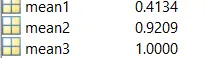
mean1=-(mean(fopt1))

figure(1)
subplot(2,1,1)
hold on
surfc(x,y,-f)
shading interp
plot3(xopt1,yopt1,-fopt1,'marker','o','markersize',5,'markerfacecolor','r');
title('Unbounded inputs')
xlabel('X-Axis')
ylabel('Y-Axis')
subplot(2,1,2)
plot(fopt1)
xlabel('Iterations')
ylabel('Function minimum')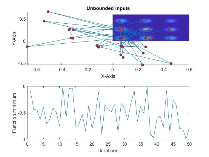

Code explanation

• In this study, we introduce the number of cases that ga needs to perform, and based on the mean value we need to calculate our global maximum value.
• We define it as num_cases=50 in this program. The 50 indicates that 50 times the ga need to repeat and it calculates the value.
• The tic command is used in order to find out the time taken for the program to complete.
• For loop command is used and the length of it set as the number of cases.
• Then ga command is used as before by calling the function and the number of variables in the program.
• The calculated x and y values are stored in xopt(i) and yopt(i).
• subplot command is used in order to get n number of plots in the same single figure plot.
• In the first plot, we plot the x,y, and f as a surface like structure by using the surf command.
• The negative sign is used in the function (f) while plotting since we invert initially and we need to revert it back to its original structure.
• Then we plot calculated maximum value as a dot-like structure by using the marker opting and marker size.
• In the next step title for the is mentioned using the title command.
• Then subplot command is used in order to plot in the same figure window.
• In this plot, we plot the values and the number of iterations, and the x label and y label is mentioned.
• In this study, we get a random value and we didn't get an exact global maximum value and the search space of ga is also not within our search space.
• Thus it indicates we need to have a better study method through which we get our exact global maximum value within our search space.

Statical case with Bounded GA

Here in the GA syntax the lower and upper bounds are defined

With defined bounds of x from '0 to 0.4' and bounds y from '0 to 0.4' better bounds results in better optimization.

%study-2 statistical behavior with upper and lower bounds

tic
for i=1:num_cases
    [inputs2,fopt2(i)]=ga(@stalagmite,2,[],[],[],[],[0,0],[1,1]);
    xopt2(i)=inputs2(1);
    yopt2(i)=inputs2(2);
end
study2_time=toc;
mean2=-(mean(fopt2))


figure(2)
subplot(2,1,1)
hold on
surfc(x,y,-f)
shading interp
plot3(xopt2,yopt2,-fopt2,'marker','o','markersize',5,'markerfacecolor','r');
title('Bounded inputs')
xlabel('X-Axis')
ylabel('Y-Axis')
subplot(2,1,2)
plot(fopt2)
xlabel('Iterations')
ylabel('Function minimum')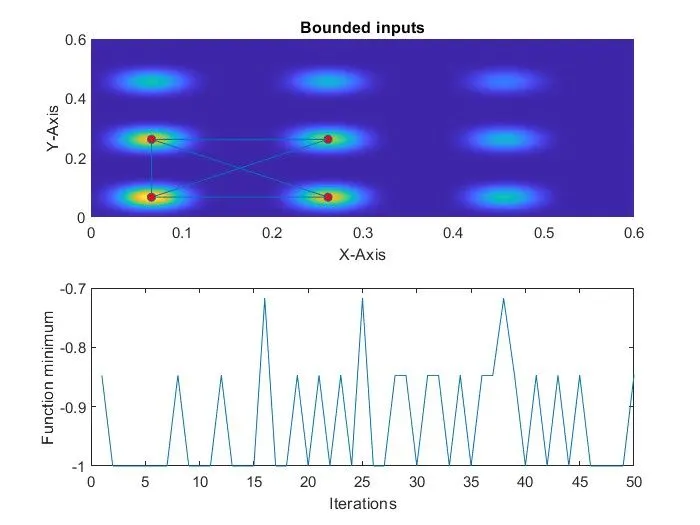

Code explanation

• From the previous study, we inferred that the search space of the ga is not within our search space so to overcome this error we use the bounded script method.
• As the name suggests, in this study we will enter the boundary and within that boundary, only the ga will perform.
• All the commands used in this study are also the same as used in the previous study except the ga syntax.
• In this study as mentioned above the limit criteria, Initially, we call the stalagmite function and the number of variables mentioned as done earlier, and we enter the lower and upper boundary limit values.
• In our program, the lower boundary limit is set as 0,0 and the upper boundary limit is set as 1,1.
• After this, we plot the same way as before and we get our plot.
• Based on the output we inferred that even though this study is better than our previous study but still we didn't an exact single global maximum value.

Statical study with Increasing Population size

Population denotes the number of data points intialieed in the space of the simulation

The default population size of the GA solver is 50.

Population size can be added as an the feature using options in the ga syntax

Increase the population size until the sigle optimum point is achieved

Increasing in the population size will incrase simulation time

Statical study Increasing Population size

%study-3 Increasing GA iterations

options=optimoptions('ga');
options=optimoptions(options,'populationsize',400);


tic
for i=1:num_cases
    [inputs3,fopt3(i)]=ga(@stalagmite,2,[],[],[],[],[0,0],[1,1],[],[],options);
    xopt3(i)=inputs3(1);
    yopt3(i)=inputs3(2);
end
study3_time=toc;
mean3=-(mean(fopt3))

figure(3)
subplot(2,1,1)
hold on
surfc(x,y,-f)
shading interp
plot3(xopt3,yopt3,-fopt3,'marker','o','markersize',5,'markerfacecolor','r');
title('Bounded inputs with modified population size')
xlabel('X-Axis')
ylabel('Y-Axis')
subplot(2,1,2)
plot(fopt3)
xlabel('Iterations')
ylabel('Function minimum')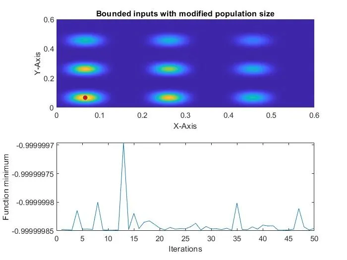

Code explanation

• In the previous study, we set the lower and upper boundary limits but we didn't set the initial population size for the ga to perform.
• Thus in this optimization technique, we will try to set the initial population size that ga needs to perform within our boundary limits.
• Thus to set the initial population size we use the optimoptions command and in that we mention the options, population size.
• After this, we plot the same way as before and we get our plot.
• The population value is randomly increased up to which a single exact global maximum value is found out.

Note :gaplotbestf, which plots the best and mean score of the population at every generation. Also setting gaplotstopping, which plots the percentage of stopping criteria satisfied.

% creating the mesh

x=linspace(0,0.6,150);
y=linspace(0,0.6,150);
 [xx,yy]=meshgrid(x,y);
 
%% for plotting the surface of stalagmite

 for i=1:length(xx)
     for j=1:length(yy)
         input_vector(1)=xx(i,j);
         input_vector(2)=yy(i,j);
         f(i,j)=stalagmite(input_vector);
     end
 end
 
 surfc(xx,yy,-f)
 shading interp
%% evalutaing the function

    options=optimoptions('ga','PlotFcn',{@gaplotbestf,@gaplotstopping},'populationsize',170);
    [x,fval]=ga(@stalagmite,2,[],[],[],[],[0;0],[1;1],[],options)
    
        xopt=x(1);
        yopt=x(2);
        
            figure(1)
            hold on
            plot3(xopt,yopt,-fval,'ro','markersize',5,'markerfacecolor','r')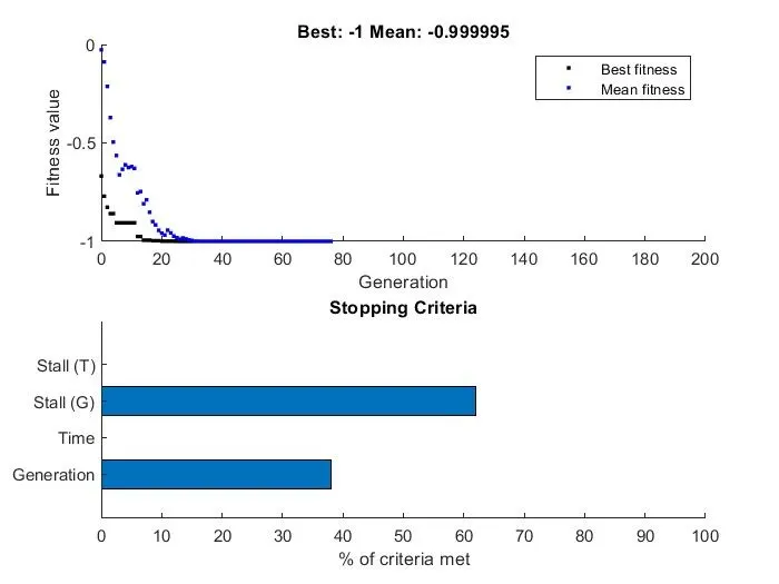

Conclusion

The Global Maxima is calculated by Population Sizing and the plots provide a visual context of the solution and verifies the authenticity of the obtained value.

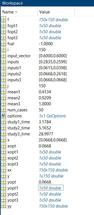
The time taken for the study, Global Maximum value and the coordinate values of x and y are found out for each study and the results are shown below

Study time

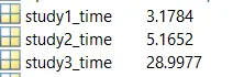
Mean