Project
- Q) Carry out a system-level simulation of an all-terrain vehicle.
Prepare a technical report explaining the model properties & comments on the results.
Aim of the Project
(i) To study the longitudinal dynamics: Vehicle speed and Displacement of an All Terrain Vehicle under various input conditions: Throttle input, Brake input, CVT gear ratio.
(ii) To study the CVT shaft speed (primary and secondary) under different CVT gear ratios.
The input conditions are provided in the following ways
a) Signal builder
b) Dashboard (Input is provided while simulation runs)
C) Lookup table (import data into lookup table for CVT gear ratio)
Based on the above input conditions, the following simulation models are run
Signal builder input for CVT gear ratio
(i) CVT model (signal builder input for throttle and CVT gear ratio)
(ii) CVT model with dashboard (Dashboard input for throttle while simulation runs and signal builder input for CVT gear ratio)
Lookup table input for CVT gear ratio
(iii) CVTmodel_CVTratio_Rpm
(iv) CVTmodel_data & Lookup table visualisation
(v) CVTmodel data mapped
(vi) CVTmodel data dashboard mapped
Before we proceed with the simulation runs and analysis of results, let us first know what an All Terrain vehicle is
All Terrain vehicle
An all-terrain vehicle (ATV) is defined as a motorized off-highway vehicle designed to travel on four low-pressure three or four tyres, having a seat designed to be straddled by the operator and handlebars for steering control. ATVs are not “one size fits all.” The ATV industry recommends all riders operate an ATV intended for their age. Youth model ATVs are designed for smaller hands and feet, and travel at slower speeds appropriate for their age.

Tyre pressure
Just changing your tire pressure one psi can make a big difference in how your ATV handles.
High tyre pressure
A higher tyre pressure is better if the purpose is to ride with multiple people on one ATV or to carry extra load.
Benefits
Higher speeds
Protects tire and rim from impacts
Great for heavier riders or carrying extra weight
Good for packed down trails
Low tyre pressure
A lower tyre pressure is extra useful for places such as, sandy areas or areas with loose dirt or gravel. If it is a requirement ride through a lot of muddy terrain, a lower tyre pressure might be something to consider as well.
Benefits
Better traction
Great for cleared trails (no smashing into boulders or tree roots)
Good for light weight riders
Great for loose terrain
System level Simulation runs
(i) CVT model (signal builder input for throttle and CVT gear ratio)
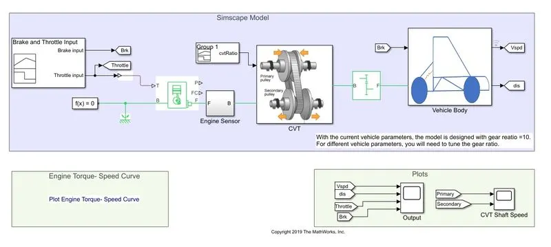
Model Properties and connections for all the blocks in the simulink model
1) Signal builder
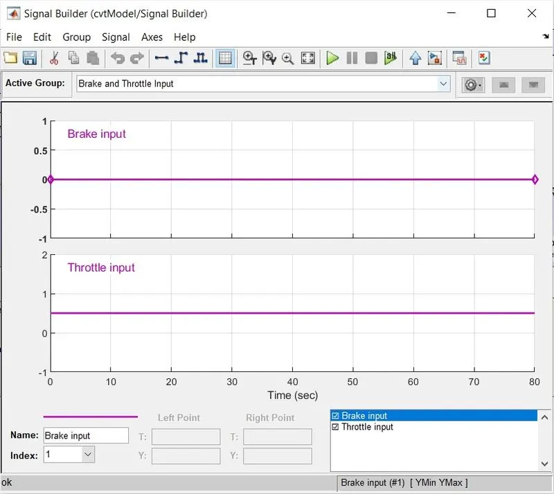
This block is used to generate input signals for brake input and throttle input.
Inputs: Throttle input is given as 0.5 from the start of the vehicle and maintained constant throughout the running time of the vehicle
Brake input is zero i.e., no brakes are applied on the vehicle throughout the running time of vehicle.
Constant sinple gear ratio = 10 and
CVT gear ratio is given as continuous signal and is as follows
2) Generic engine or Engine block
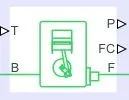
Represents a system-level model of spark-ignition and diesel engines suitable for use at initial stages of modeling when only the basic parameters are available. Optional idle speed and red line controllers are included.
The throttle input signal T lies between zero and one and specifies the torque demanded from the engine as a fraction of the maximum possible torque. If the engine speed falls below the Stall speed, the engine torque is blended to zero. If the engine speed exceeds the Maximum speed, the simulation stops and issues an error message.
Connections F and B are mechanical rotational conserving ports associated with the engine crankshaft and engine block, respectively. Connections P and FC are physical signal output ports through which engine power and fuel consumption rate are reported.
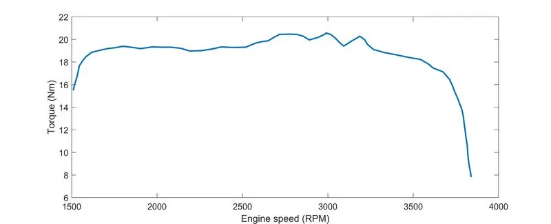
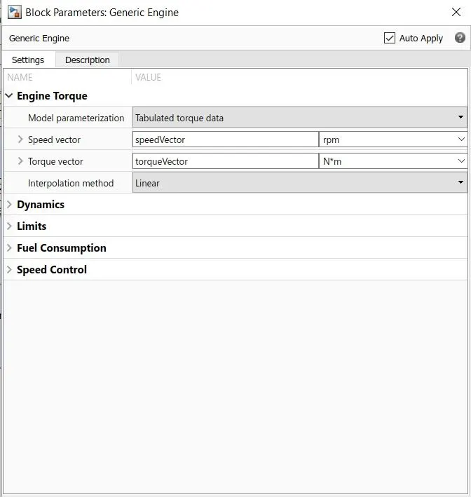
The torque vector data and speed vector data are imported from the practical approach using BAJA ATV. The vehicle is accelerated from 0 to a threshold rpm without braking or decelerating and, the torque data (against engine rpm) and the speed data(against engine rpm) are recorded.
3) Engine sensor subsystem
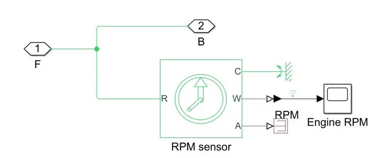
An ideal rotational motion sensor is used to record or detect the rpm of the engine crankshaft.
The physical signal ports W and A report the angular velocity and angle, respectively, of port R relative to port C. The measured angular velocity is positive when the angular velocity at port R is greater than the angular velocity at port C. Port C is stationary and therefore connected to fixed rotational reference frame. Port W is connected to scope as the requirement is to observe the variation of rpm w.r.t to time.
Port A is connected to PS terminator as there is no requirement of observing the variation of angle w.r.t time.
4) CVT subsystem
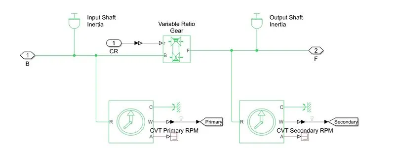
CVT or Continuous Variable Transmission is an automatic gear transmission system that has infinite gear ratios , the gear ratio varies continuously and smoothly based on the throttle input.
In Simulink, CVT gear ratio is provided as input to variable gear ratio block. Based on this input , the CVT subsystem generates an output velocity using two pulleys and belt system.
R is the input port that receives engine rpm, B is base – primary pulley or shaft, F is follower – secondary pulley or shaft.
Input shaft inertia represents primary shaft connected to B of port and output shaft inertia represents secondary shaft to which the F port is connected.
Ideal rotational motion sensors are used to detect rpm of primary and secondary shafts.
5) Simple Gear

The secondary shaft is connected to base port of simple gear block and is subjected to reduction gear ratio of 10 and the output follower port F is connected to wheels of the ATV.
6) Vehicle body subsystem
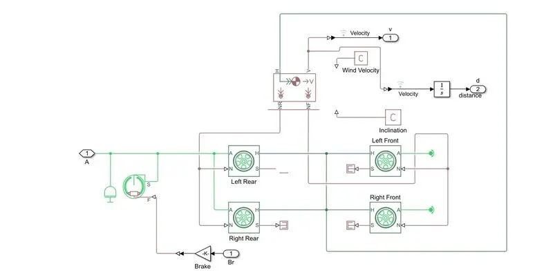
The output rpm from the follower of simgle gear is connected to wheel shaft using inertia shaft block. This in turn is connected to front wheels of the vehicle.
Wheel block and Vehicle block connections to solve for vehicle velocity
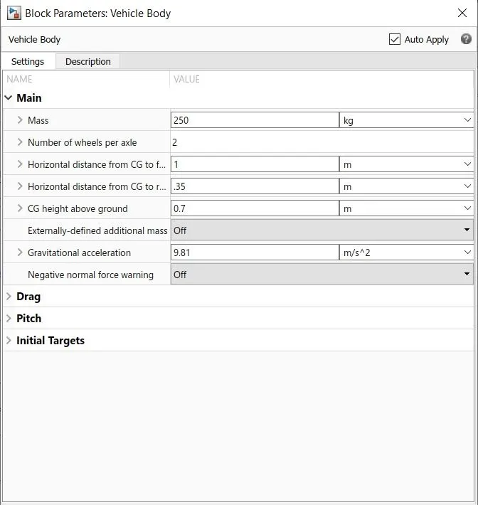
It can be seen from the vehicle block parameter window that tractive force and normal force inputs are not given for vehicle, the governing equation for longitudinal vehicle i.e.,

requires these inputs to solve for vehicle velocity (Fx - tractive force). Therefore, inputs are given by connecting the vehicle block to the wheel block and the connections are as follows
The wheel block port A is rotational conserving port and for front wheels, input rpm is provided from shaft. The A port of rear wheels is connected to free end as they are driven by front wheels. The wheel block port H is translation mechanical port, this port is connected to H port of the vehicle. As the tyres apply force on the road, a reaction for will be generated on the vehicle that makes the vehicle to move, this is also called as tractive force. The Nf and Nr , normal reaction forces on the front and rear tyres port from vehicle body is connected to wheels N port. Nf to left and right front wheels, and Nr to right and left rear wheels.
The vehicle longitudinal dynamics governing equations require tractive force and reactive force values to solve for the velocity. These values are provide by connecting the tyres to vehicle block.
7) Double shoe brake

This block’s input port F receives signal from brake and generates a output braking on the wheel shaft. The output port S is connected to shaft inertia block.
Since all the inputs are defined for the model, now the simulation is run for a duration of 200 seconds
Results
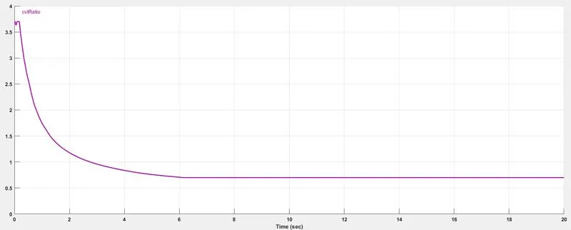
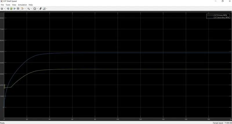
From the above plots, it can be seen that secondary shaft rpm is lower than primary shaft rpm and gradually increases and becomes greater than primary shaft rpm and remains constant throughout.
This is because of the input CVT gear ratio provided, the CVT gear ratio is high in the initial stages and decreases gradually to a lower value and remains constant throughout.
As the CVT gear ratio is high, the ratio of teeth of driven gear to teeth of driving gear is high, this infers that the speed of driven gear i.e, the secondary shaft is less compared to driving gear i.e., the primary shaft (no of teeth of gear in inversely proportional to speed of the gear). As the ratio varies from high to low, the secondary shaft rpm becomes more than primary shaft rpm and remains constant throughout.
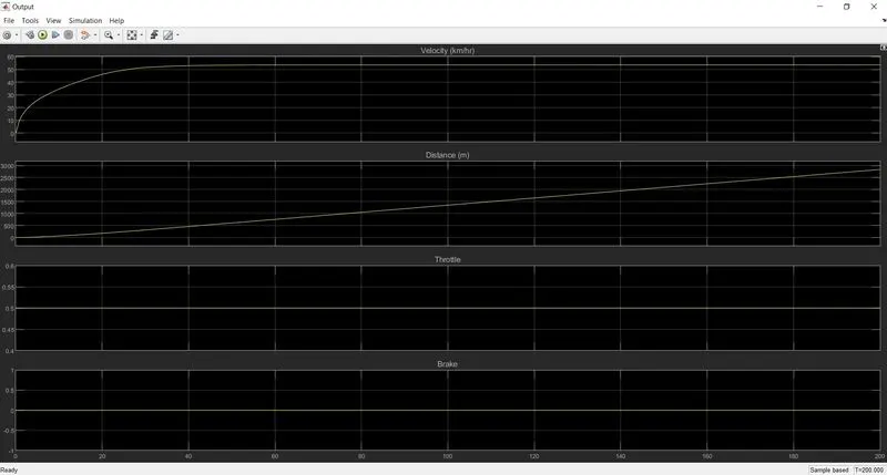
As it can be observed from the plot that the throttle input is constant, therefore, the vehicle accelerates from zero and reaches a value that matches or compatible with throttle input followed by gear ratios(CVT variable and constant simple gear) and moves with that constant or uniform velocity. Since the brake input is zero, there is no deceleration of the vehicle and the distance travelled by the vehicle increases at constant rate.
(ii) CVT model with dashboard (Dashboard input for throttle while simulation runs and signal builder input for CVT gear ratio)
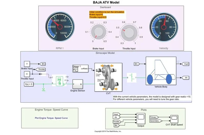
This model is similar to previous model except that the inputs are provided while simulation runs using dashboards.
Inputs: Throttle input is maintained at 0.5 and brake input given is zero, CVT gear ratio and constant simple gear ratio is same as in previous model.
simulation time: inf
Results
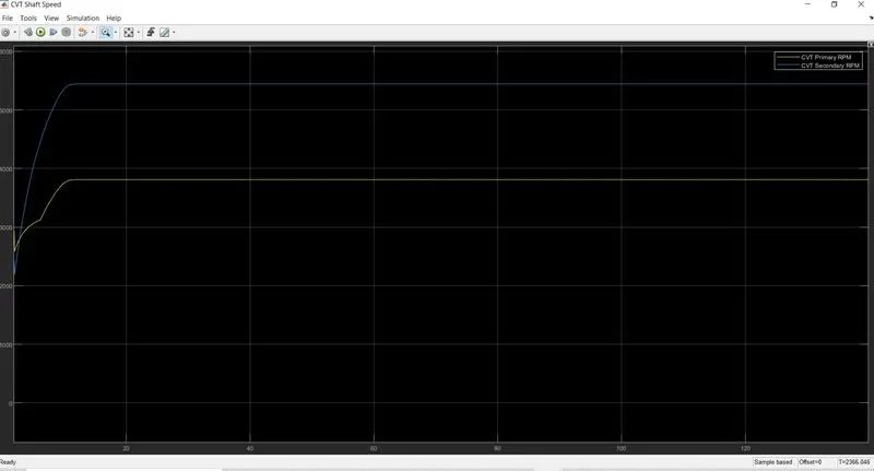
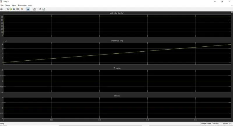 I
I
It can be seen from the above plots that the shaft speeds - primary and secondary are varying w.r.t CVT gear ratio and the vehicle velocity is dependent on the constant throttle input of 0.5 followed by gear ratio (CVT variable and constant simple gear).
(iii) CVTmodel_CVTratio_Rpm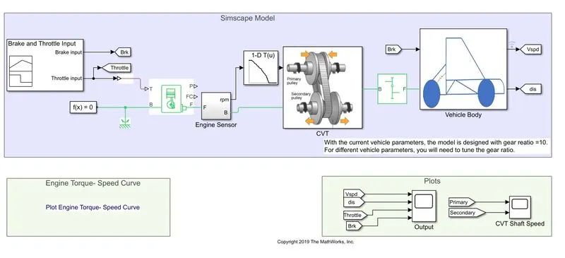
Input CVT ratio is given using engine rpm. Lookup table block is used to provide input for CVT gear ratio.
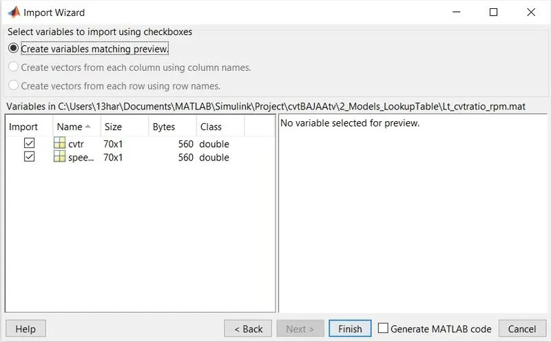
The data is imported from matlab file by defining the varibles cvtr and speedV in base workspace.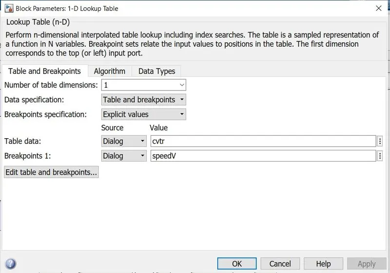
simulation time: 50s
Results
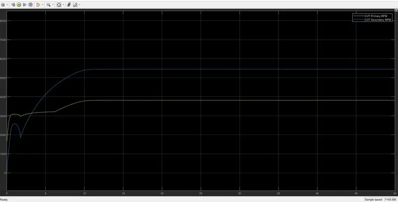
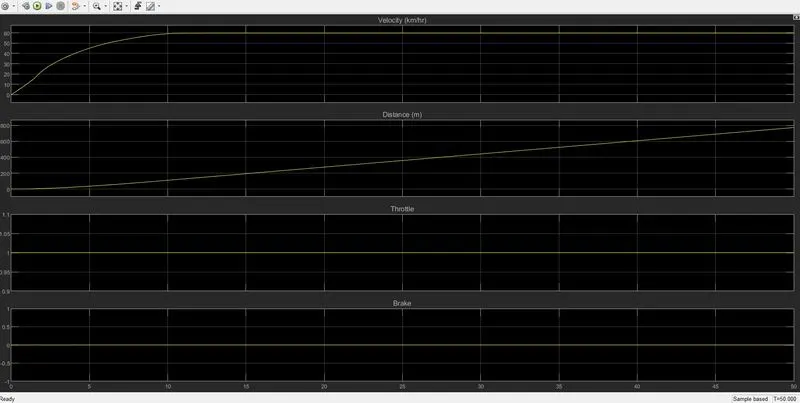
As observed from the plots, a constant throttle input of 1 is provided to the engine. The primary and secondary shaft speed behaviour is w.r.t given CVT ratio input. There is an increase in shaft speeds and the vehicle velocity as the throttle input increased by 0.5 units.
(iv) CVTmodel_data & Lookup table visualisation
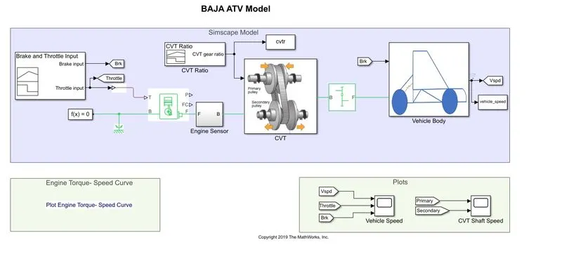
Inputs: Throttle input 0.3 for initial 20 sec and 1 for remaining time
Brake input is zero, constant simple gear ratio 12
CVT gear ratio is as follows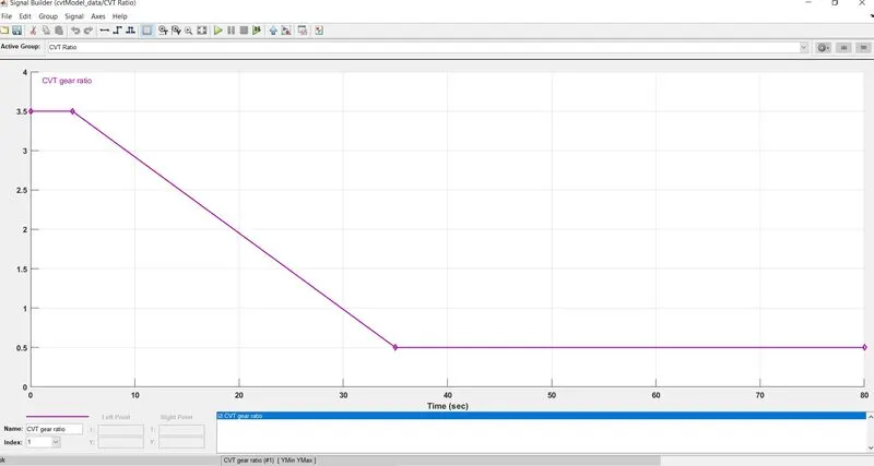
simulation time: 200s
Results
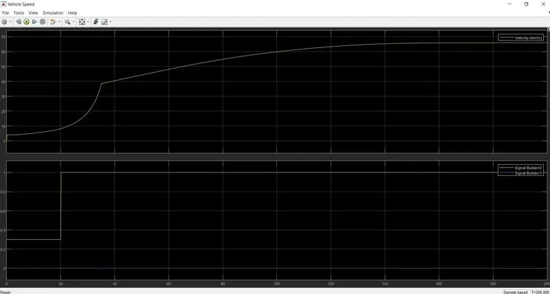
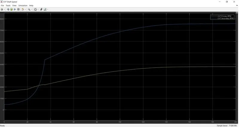
It can be observed from the plots that the velocity of the vehicle was low at for initial 20s and increased to near 70kmph. This is due to variation in throttle input after 20s.
The CVT shaft speeds varied according to the CVT gear ratio
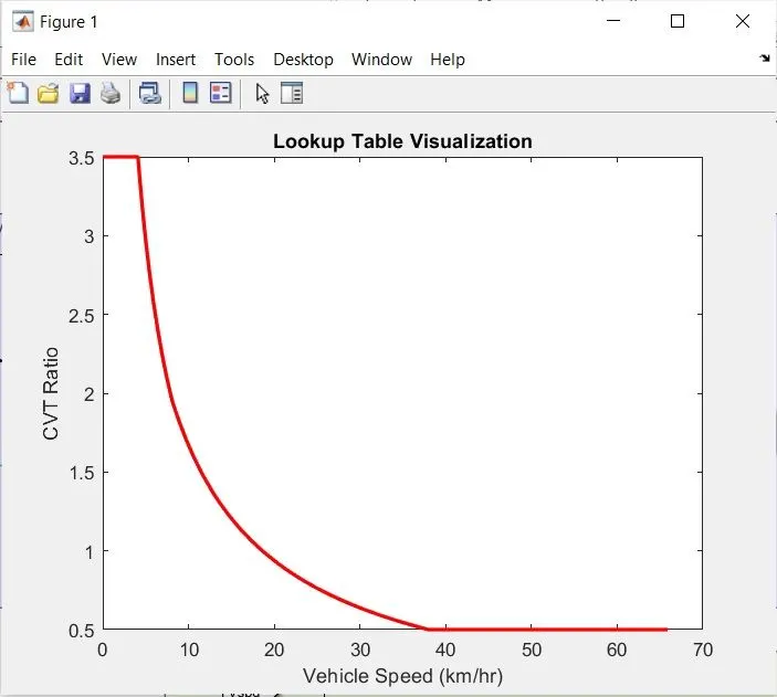
Lookup table visualisation
The cvt ratio and output velocity were stored in base workspace with variable names cvtr and velocity_speed.
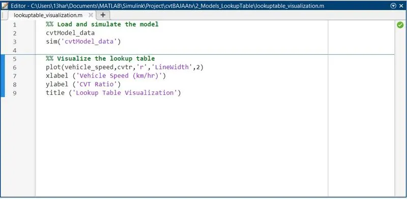
The cvtmodel is run using a script and a plot is generated to observe the variation of cvtr w.r.t velocity_speed.
(v) CVTmodel data mapped
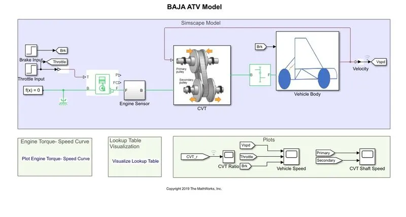
Inputs: The inputs are similar to previous model except for CVT gear ratio
The cvtr and vehicle_speed data from the previous mode (CVTmodel_data) is mapped using PS lookup table to CVT block.
It can be performed in two ways
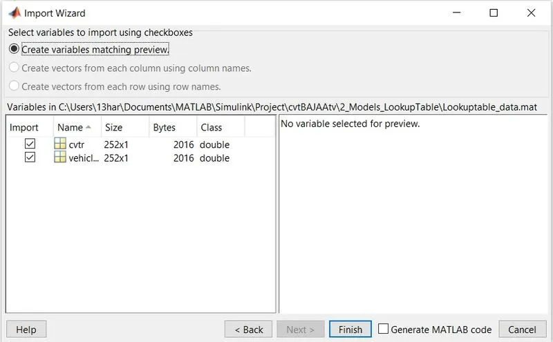
1) Using lookup table
Import data from matlab file and define in base workspace
2) Using the results of previous model i.e., cvtmodel_data that are stored in workspace
PS lookup table takes data that is strictly ascending or descending
select cvtr vector data from workspace and sort it to descending order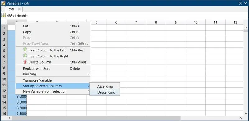
Select vehicle_speed vector data and sort it to ascending order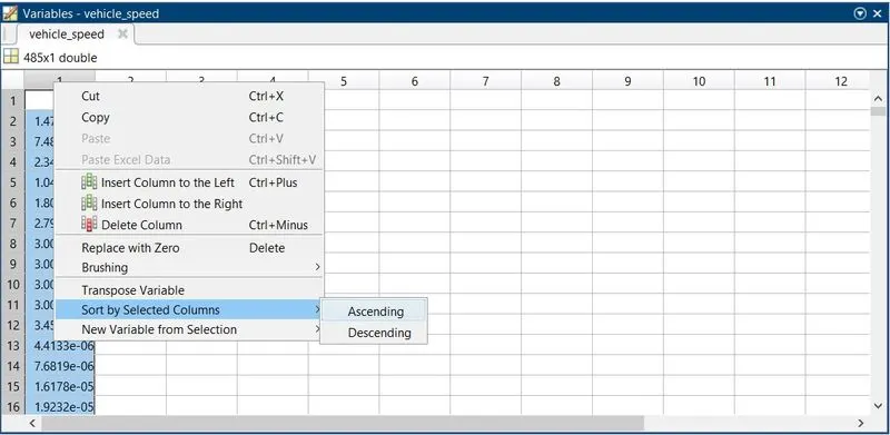
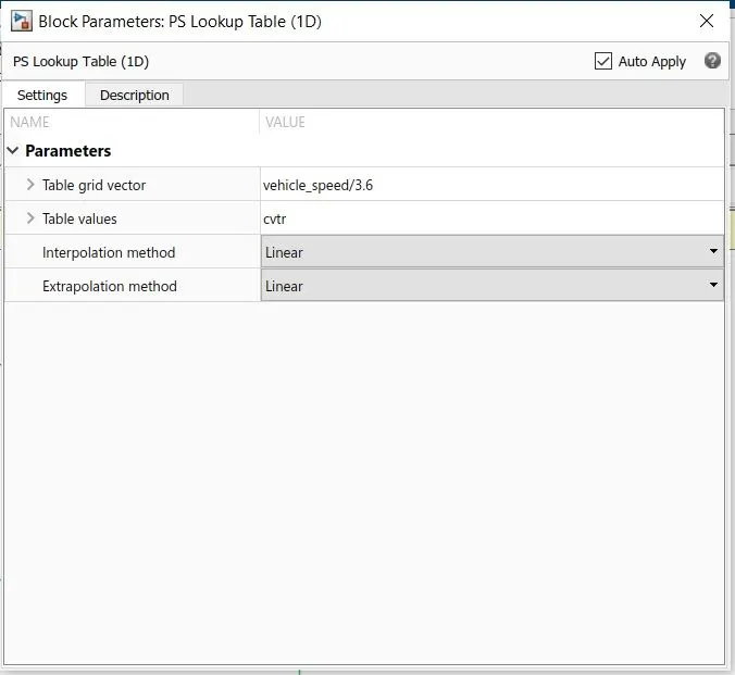
simulation time: 200s
Results
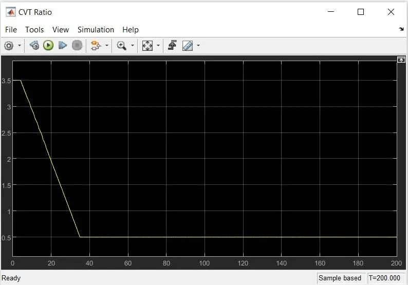
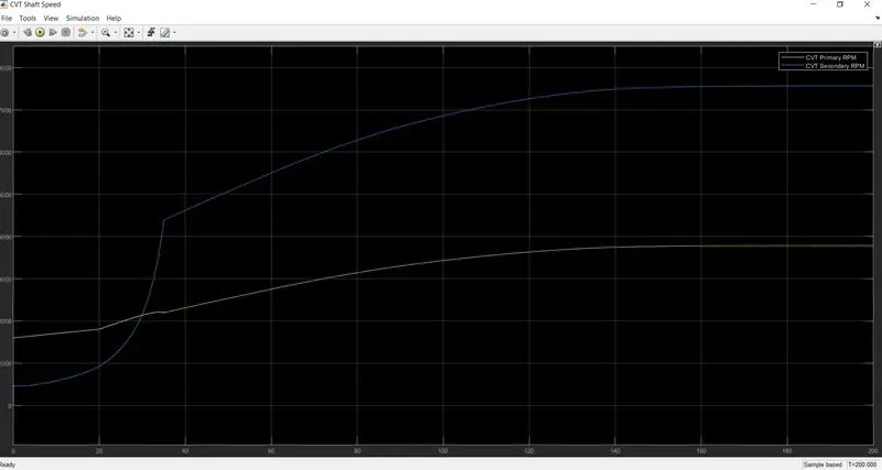
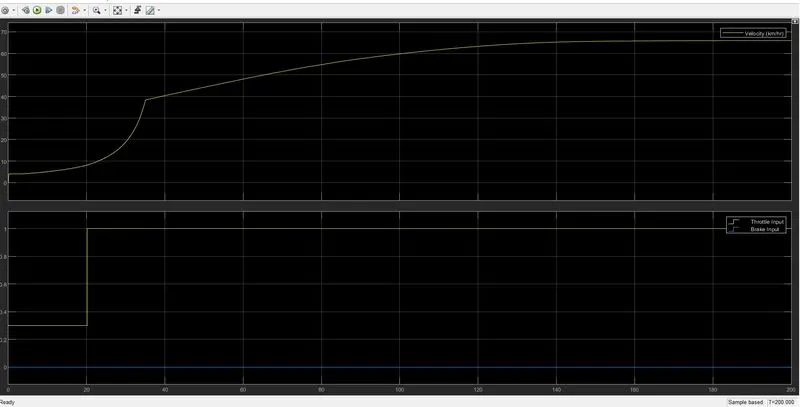
The CVT gear ratio generated is a well defined as the solver interpolates for the values that fall in between the defined or given input vector data and extrpolates for the values the fall out of range.
The CVT shaft speed variation is based on CVT gear ratio and variation Vehicle speed is w.r.t to throttle input followed by gear ratio.
(vi) CVTmodel data dashboardmapped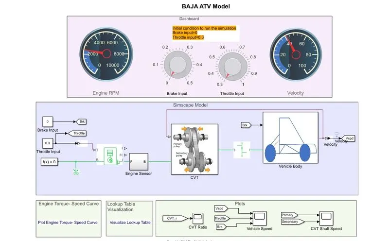
All the inputs and parameters are similar to previous model except that the input is provided using dasborads while simulation runs
The throttle input is kept constant at 0.3 and not varied.
simulation time: inf
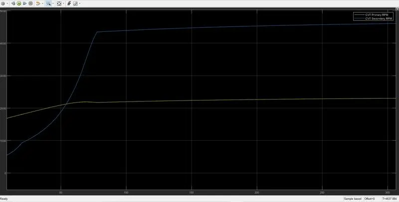
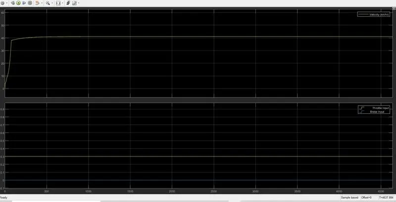
Since the throttle input is maintianed constant, the vehicle accelerates from 0 to around 40kmph and there is no change in vehicle velocity after that and remains in uniform state throughout.
System level simulation is run for all models
Model properties and results are discussed