Project

Aim: To study BAJA all-terrain vehicle (ATV) Simulink model and compare different model

Objectives:

• Prepare a technical report explaining the model properties & comments on the results.

There are 5 types of models under study which are:

• BAJA ATV model without dashboard
• BAJA ATV model (cvtModel_data)
• BAJA ATV model with dashboard (cvtModel_dashboard)
• BAJA ATV model Mapped lookup table without a dashboard
• BAJA ATV model Mapped lookup table with dashboard

Introduction to ATV:

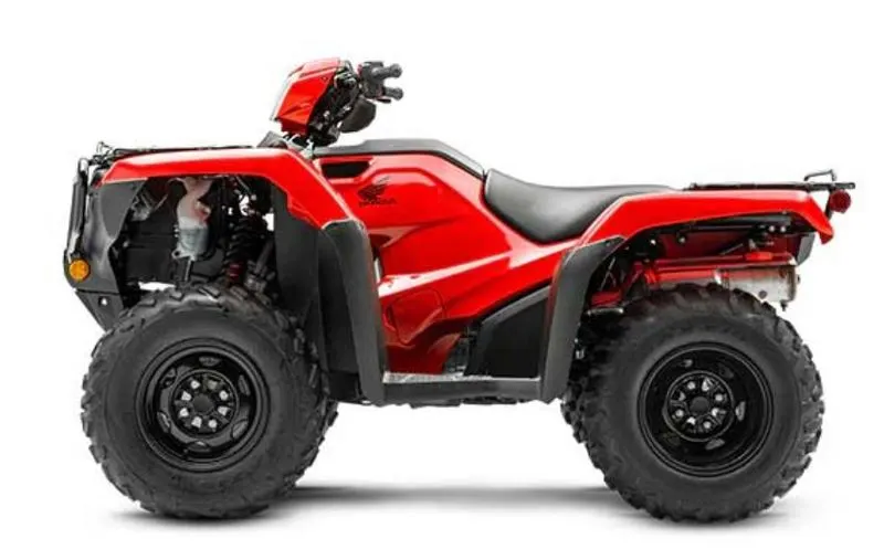
An all-terrain vehicle (ATV), also known as a light utility vehicle (LUV)a quad bike, or simply a quad, as defined by the ANSI, is a vehicle that travels on low-pressure tires, with a seat that is straddled by the operator, along with handlebars for steering control. As the name implies, it is designed to handle a wider variety of terrain than most other vehicles.

BAJA SAE:

Baja SAE is a Collegiate Design series competition run by the Society of Automotive Engineering International (SAE International). Teams of students from universities all over the world design and build small off-road cars. The cars all have engines of the same specifications. As of 2018, the engine has been an unmodified Briggs&stratton Model 19 Vanguard engine single cylinder with a displacement of 305cc and power output of approximately 10 bhp (7.5 kW).

INtroduction to CVT:

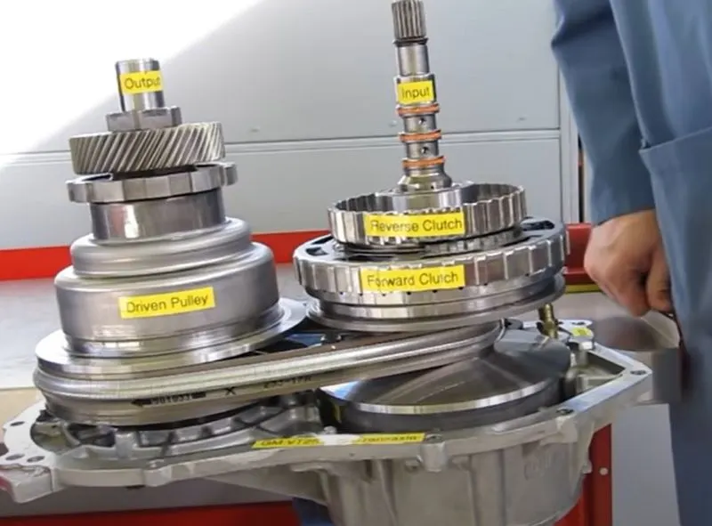
A CVT, or continuously variable transmission, seamlessly changes through an unending range of effective gear ratios while you drive, whereas other kinds of mechanical transmissions offer a fixed number of gear ratios and have hard shifts between each as explained by Certified Transmission Repair. CVT transmission systems are also known as single-speed, shiftless, and stepless transmissions. The shiftless nature of a CVT offers unparalleled flexibility that maintains constant angular velocity regardless of output speed. Additionally, a continuously variable transmission makes accelerating smooth and offers enhanced fuel economy.

In this Simulink model all the main block used are as follow:

Generic Engine Block:

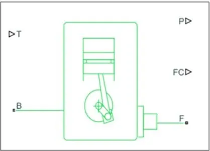
The Generic Engine block represents a general internal combustion engine. This block is a suitable generic engine for spark-ignition and diesel. Speed-power and speed-torque parameterizations are provided. A throttle physical signal input specifies the normalized engine torque. Optional dynamic parameters include crankshaft inertia and response time lag. A physical signal port outputs the engine fuel consumption rate based on the fuel consumption model that you choose. Optional speed and redline controllers prevent the engine to stall and enable cruise control.

All the ports are explained below:

• T: Engine torque demand as a fraction of maximum possible torque.
• P: Power produced by the engine, in W.
• FC: Fuel consumed by the engine, in kg/s.
• B: Mechanical rotational conserving port associated with the engine block. This is the base port. The engine block is the physical body that contains the piston cylinders.
• F: Mechanical rotational conserving port associated with the engine crankshaft. This is the follower port of the engine. The crankshaft transmits the power generated from the combustion process. Typically, you attach a clutch and transmission at this port.

Simple gear:

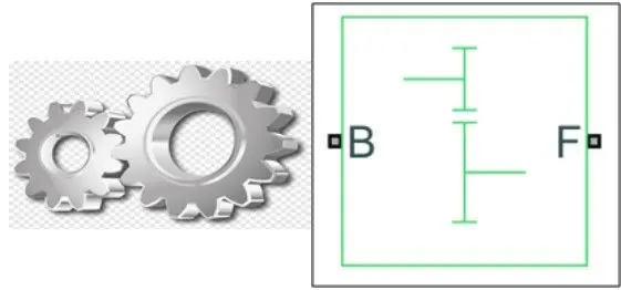
The Simple Gear block represents a gearbox that constrains the connected driveline axes of the base gear, B, and the follower gear, F, to corotate with a fixed ratio that you specify. You choose whether the follower axis rotates in the same or opposite direction as the base axis. If they rotate in the same direction, the angular velocity of the follower, ω_F, and the angular velocity of the base, ω_B, have the same sign. If they rotate in opposite directions, ω_F and ω_B have opposite signs. You can easily add and remove backlash, faults, and thermal effects.

Connections B (base) and F (follower) are mechanical rotational conserving ports. Specify the relation between base and follower rotation directions with the Output shaft rotates parameter. Optionally include thermal effects and expose thermal conserving port H by setting the Friction model to a temperature-dependent setting.

Variable Ratio Transmission block:

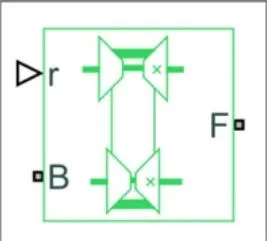
Represents a variable ratio gearbox such as implemented by mechanical belt CVT, electric, or hydraulic transmissions. The physical signal input r defines the ratio of input to output angular shaft velocities. Connections B (base) and F (follower) are mechanical rotational conserving ports. Specify the relation between base and follower rotation directions with the Output shaft rotates parameter.

Double-Shoe Brake block:

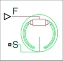
Represents a brake arranged as two pivoted rigid shoes symmetrically installed inside or outside a drum and operated by one actuator. The actuator force causes the shoes to exert friction torque on a shaft connected to the drum. Connection S is a conserving rotational terminal associated with the drum shaft. Connection F is a physical signal port representing the force input to the actuator. Positive force creates friction torque that resists shaft rotation. Optionally include thermal effects and expose thermal conserving port H by setting Thermal port to Model.

Tire (Magic Formula) block:

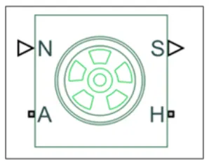
Represents the longitudinal behavior of a highway tire characterized by the tire Magic Formula. The block is built from Tire-Road Interaction (Magic Formula) and Simscape Foundation Library Wheel and Axle blocks. Optionally, the effects of tire inertia, stiffness, and damping can be included. Connection A is the mechanical rotational conserving port for the wheel axle. Connection H is the mechanical translational conserving port for the wheel hub through which the thrust developed by the tire is applied to the vehicle. Connection N is a physical signal input port that applies the normal force acting on the tire. The force is considered positive if it acts downwards. Connection S is a physical signal output port that reports the tire slip. Optionally expose physical signal port M by setting Parameterize by to Physical signal Magic Formula coefficients. Physical signal port M accepts a four-element vector corresponding to the B, C, D, and E Magic Formula coefficients.

Vehicle body block:

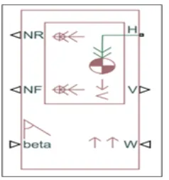
Represents a two-axle vehicle body in longitudinal motion. The block accounts for body mass, aerodynamic drag, road incline, and weight distribution between axles due to acceleration and road profile. The vehicle can have the same or a different number of wheels on each axle. Optionally include pitch and suspension dynamics or additional variable mass and inertia. The vehicle does not move vertically relative to the ground. Connection H is the mechanical translational conserving port associated with the horizontal motion of the vehicle body. The resulting traction motion developed by tires should be connected to this port. Connections V, NF, and NR are physical signal output ports for vehicle velocity and front and rear normal wheel forces, respectively. Wheel forces are considered positive if acting downwards. Connections W and beta are physical signal input ports corresponding to headwind speed and road inclination angle, respectively. If the variable mass is modeled, the physical signal input ports CG and M are exposed. CG accepts a two-element vector representing the x and y distance offsets from vehicle CG to additional load mass CG. M represents the additional mass. If both variable mass and pitch dynamics are included, the physical signal port J accepts the inertia of the additional mass about its own CG

BAJA ATV MODEL WITHOUT DASHBOARD:

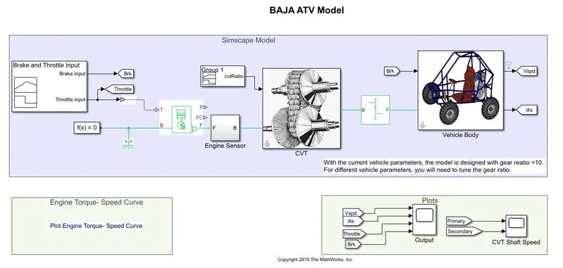
Model explanation:

• Throttle signal generated by signal builder block and given to the genric engine block
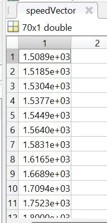
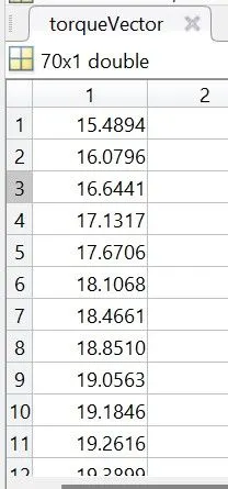
• Torque and speed vector is given to the engine from the model workspace
• 
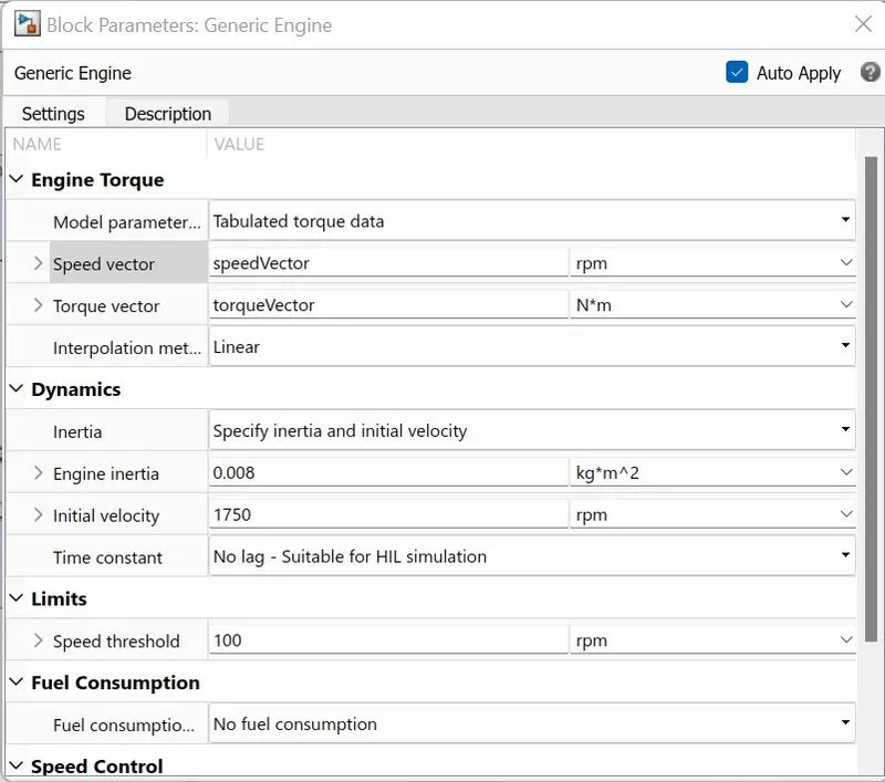
• The engine will generate output RPM at the crankshaft and this output is given to the ideal rotational motion sensor to sense the output RPM
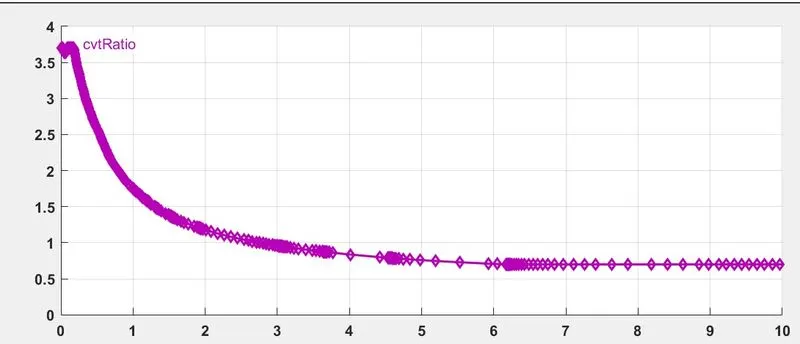
• The same output is given to the Variable ration transmission block (CVT), the CVT ratio is provided to this block through the signal builder
• The output speed of the variable transmission block is given to a simple gear mechanism where the gear ratio is 10, and this controlled output speed is given to the vehicle axel
• The break signal generated by signal block is given to the vehicle body via a double shoe brake to apply a brake to the axel
• The velocity and distance are taken as the output of the vehicle body for further analysis.

Input signals:

Throttle input signal:;

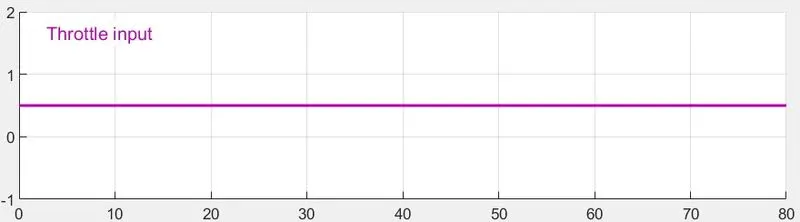
Throttle input remains 0.5 for the whole simulation.

Brake input signal:

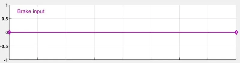
Brake input remains zero for the whole simulation.

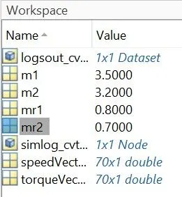
Matlab workspace inputs-

CVT ratio input-

Engine sensor sub-block-

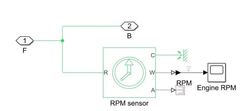
This sub-block measures engine rotation speed by ideal rotational motion sensor.

CVT sub-block:

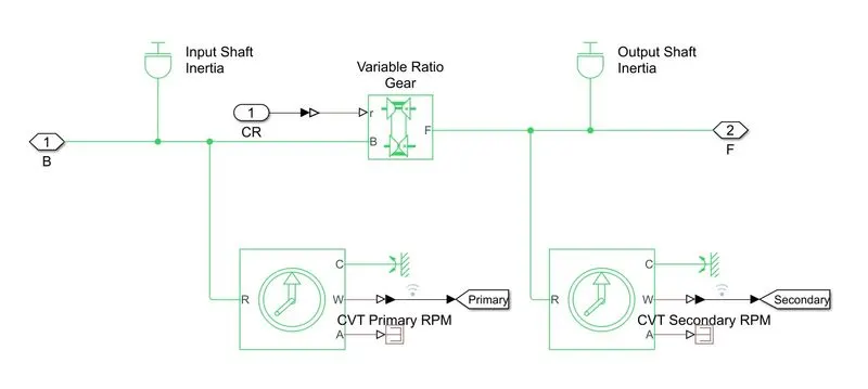
In this block, both input and output shaft is provided inertia and and with ideal rotational motion sensor primary and secondary shaft rpm is measured.

Vehicle body sub-block-

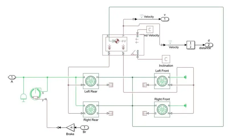
As we can see in the sub-block vehicle is rear-wheel drive as the output from the gearbox is inputted to rear axels, also inertia is given to the axel, and shoe brake s port is connected to the axle and then the same axel is connected to the rear wheels and brake signal is given to f port of shoe brake through gain to simulate small movement in the brake pedal create large brake force. front tyres rotate freely on rotation free end, all the tyres Hub H port is connected together and connected to vehicle H port, also normal force N port of rear tyres is connected to Nr port of the vehicle and same for Nf port, also for vehicle road inclination and wind velocity is taken as constant.

Engine RPM plot:

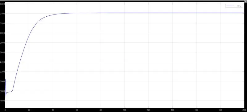
As we can see from the plot engine rpm is generated according to throttle and speed and torque vectors, engine accelerates from 1800 to 3400 rpm for first 20 sec and then remains constant for rest of the simulation

Vehicle speed and distance plot:

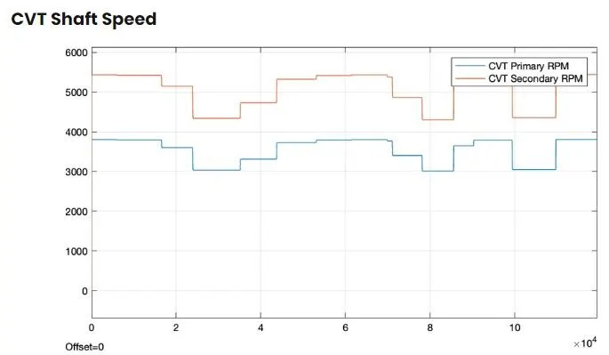
CVT shafts speed plot:

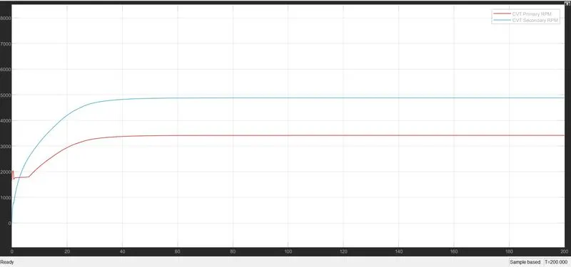
We can see variations in primary and secondary shaft rpm according to their gear ratios

Case 2: All-terrain vehicle (ATV) with Dashboard:

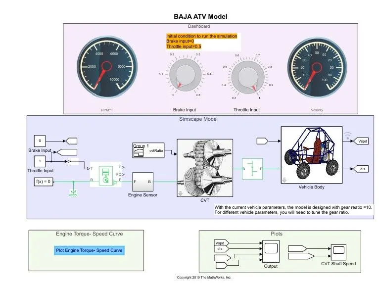
Model explanation:

• This model is the same as the previous edition of the dashboard which has a Brake and Throttle Input knob that allows the user to change the input values in running the simulation
• We kept the brake input as zero and change the throttle input as per the users will, which changes vehicle speed simultaneously.

CVT ratios-

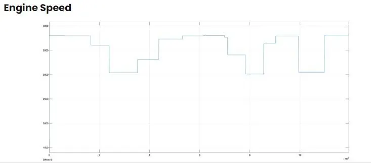
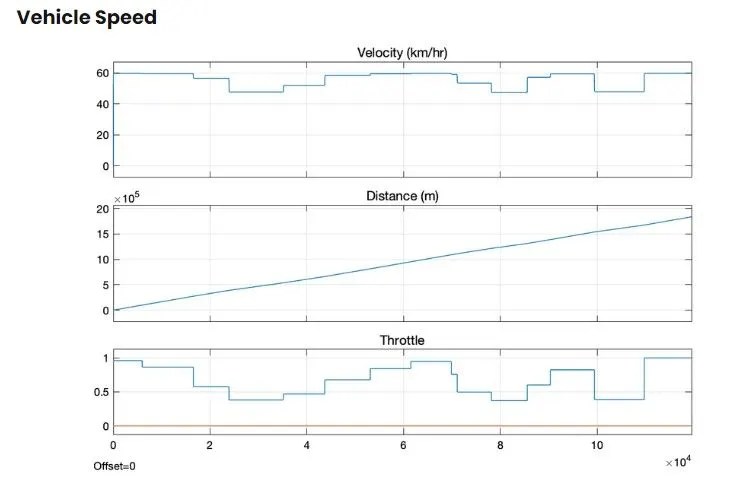
As we can see from the plot change in throttle input reflects on vehicle speed.

Case 3: All-terrain vehicle with a lookup table

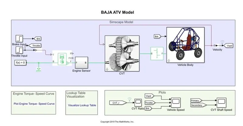
Model explanation:

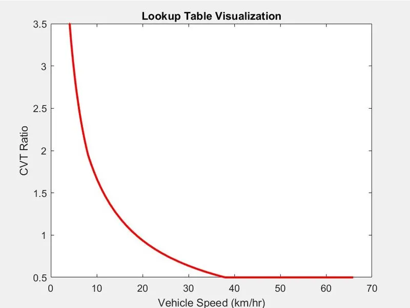
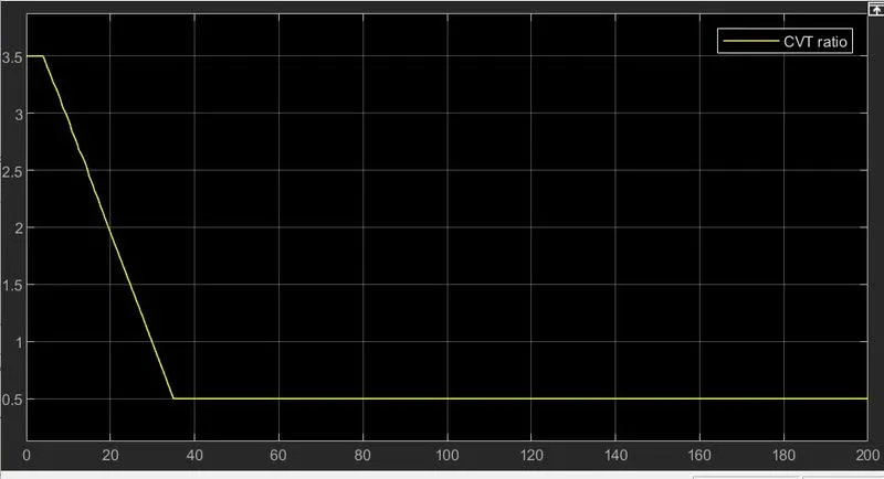
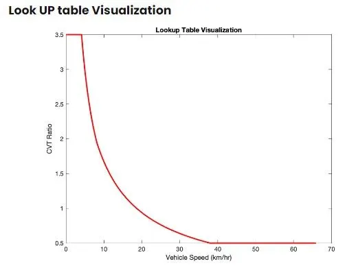
• Here brake and throttle step signal is used as input, lookup table with CVT ratio and vehicle speed as a visualization table helps to specify the CVT ratio
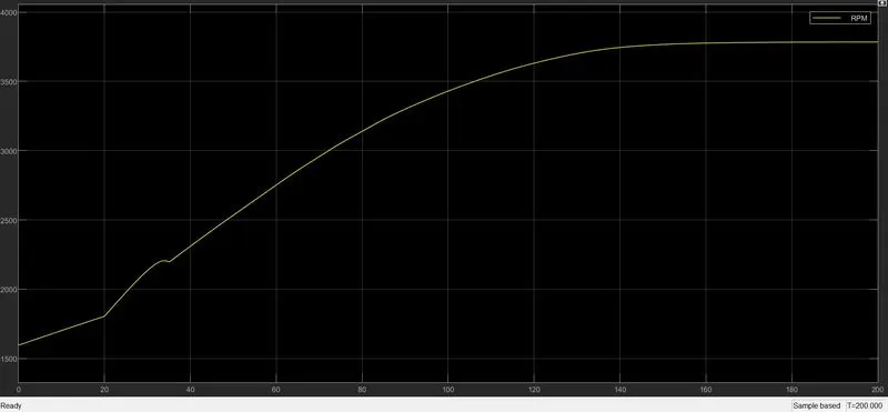
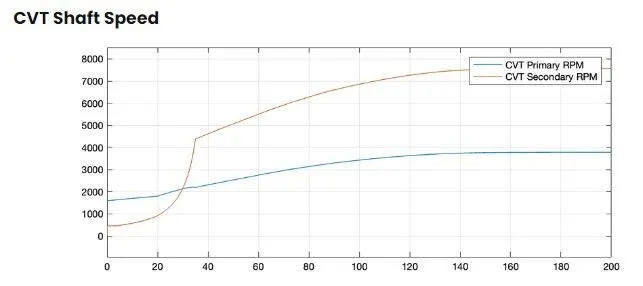
• We run this simulation for 200 sec which gives output in form of various plots which are engine rpm, vehicle speed, speed of the primary and secondary shaft of CVT

Results:

Lookup table

CVT ratio:

Engine RPM:

Vehicle speed:

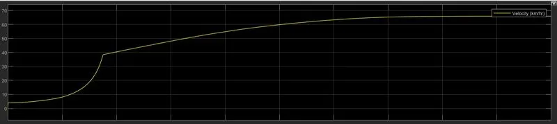
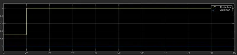
Here as we can see that brake input is kept at 0, while throttle input is at 0.3 between 0 to 20 sec, and then at 1 for the rest of the simulation, Vehicle speed also shows a gradual growth in the first 20 sec and later increase from in 20 to 40 sec and gets stablled.

CVT shaft speed-

Case 4: All-terrain vehicle with a dashboard using a Lookup table

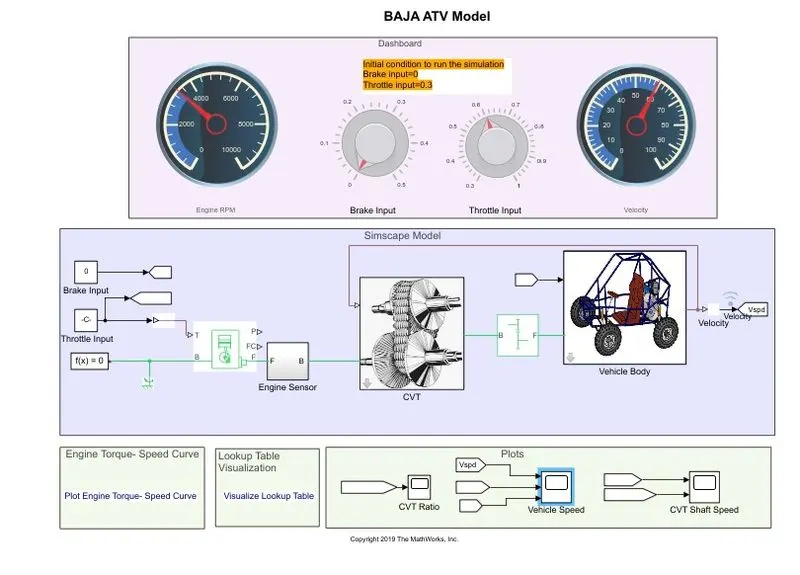
Model explanation:

• Here Model is similar to the previous model with the edition of the dashboard along with look up table
• Here input can be given using knobs for throttle and brake, making changes there will simultaneously change vehicle speed
• Here we kept brake input as 0 and the throttle can be changed with the knob according to the user

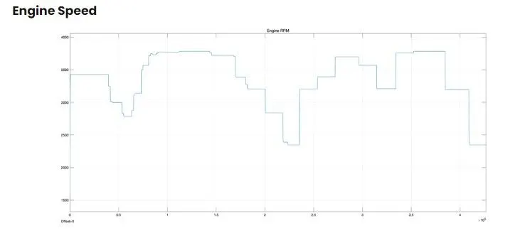
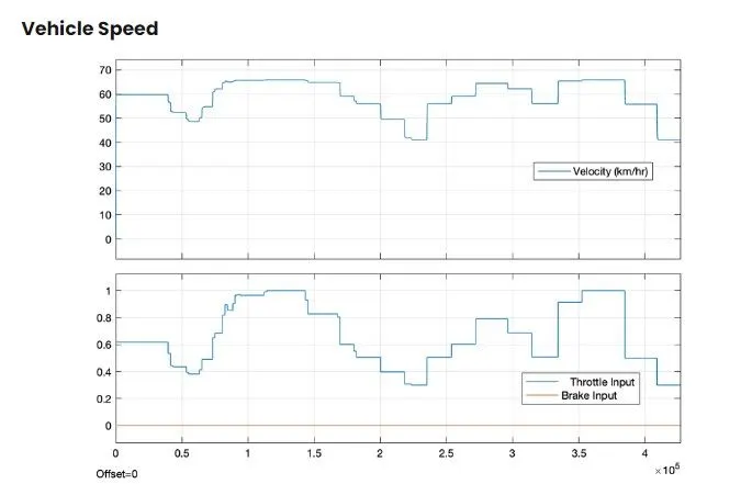
In the graph, we can see that increase in throttle input increases vehicle speed and vice versa for falls in the throttle input, the brake remains zero for all the simulation

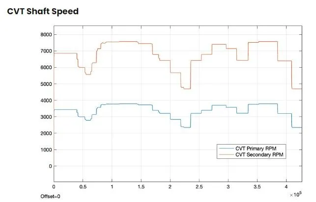
Here we can see that Changes in primary and secondary shaft speed as per the gear ratio

Reference:

Matlab help

Github files