Week 3 - Solving second order ODEs

AIM: To create an animation on a simple pendulum by solving second order differential equation which represents the motion of simple pendulum with damping using ODE solver functions

Solution:

In the above equation,

g = gravity in m/s2,

L = length of the pendulum in m,

m = mass of the ball in kg,

b=damping coefficient.

L=1 metre,

m=1 kg,

b=0.05.

g=9.81 m/s2.

Simulate the motion between 0-20 sec, for angular displacement=0,angular velocity=3 rad/sec at time t=0.

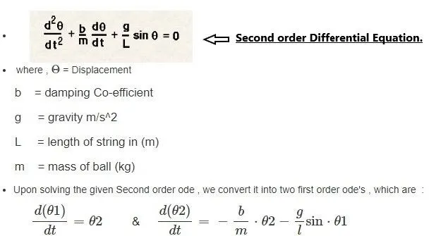
In order to solve second order ode in MATLAB, we have to convert it into first-order ODEs

program for ODE function

function [dtheta_dt]= ode_func(t,theta,b,g,l,m)
theta1= theta(1)
theta2= theta(2)
dtheta1_dt= theta2;
dtheta2_dt=-(b/m)*theta2-(g/l)*sin(theta1);
dtheta_dt=[dtheta1_dt;dtheta2_dt];
end

Main Program:

clear all
close all
clc

%Defining inputs
b=0.05;
g=9.81;
l=1;
m=1;

%initial condition
theta_0=[0;3];

%time span
t_span=linspace(0,20,300);

%slove ODE
[t,results]=ode45(@(t,theta) ode_func(t,theta,b,g,l,m),t_span,theta_0);

plot(t,results(:,1))
hold on

plot(t,results(:,2))
legend('displacement','angular velocity')

% For animating the motion of pendulum
figure(2)
ct=1
for i=1:length(results(:,1))
    x0=0;
    y0=0

    x1=l*sin(results(i,1));
    y1=-l*cos(results(i,1));

    plot([0 0],[-1.5 0.5])
    hold on
    plot([x0 x1],[y0,y1],'LineWidth',1,'Color','b')
    axis([-1.5 1.5 -1.5 0.5])
    plot(x1,y1,'o','MarkerSize',20,'Color','r')
    pause(0.0001)
    M(ct)=getframe(gcf)
    hold off
    ct=ct+1
end

%making a video file
movie(M)
videofile=VideoWriter('simple_pendulum.avi','Uncompressed AVI')
open(videofile)
writeVideo(videofile,M)
close(videofile)

Code Explanation:

clear all
close all
clc

%Defining inputs
b=0.05;
g=9.81;
l=1;
m=1;

%initial condition
theta_0=[0;3];

%time span
t_span=linspace(0,20,300);

Here we define all the inputs provided in a question and define the initial condition and time span

%slove ODE
[t,results]=ode45(@(t,theta) ode_func(t,theta,b,g,l,m),t_span,theta_0);

plot(t,results(:,1))
hold on

plot(t,results(:,2))
legend('displacement','angular velocity')

Here we solve the ode_fun we defined earlier by using 'ode45' solver.

ode45: Is a solver whose function which solves ordinary or partial differential equations using numerical method (Range Kutta method) here 'ode45' integrates the function which f(t,theta) from (t0,tf) i.e. (0 to 20) with initial conditions theta_0

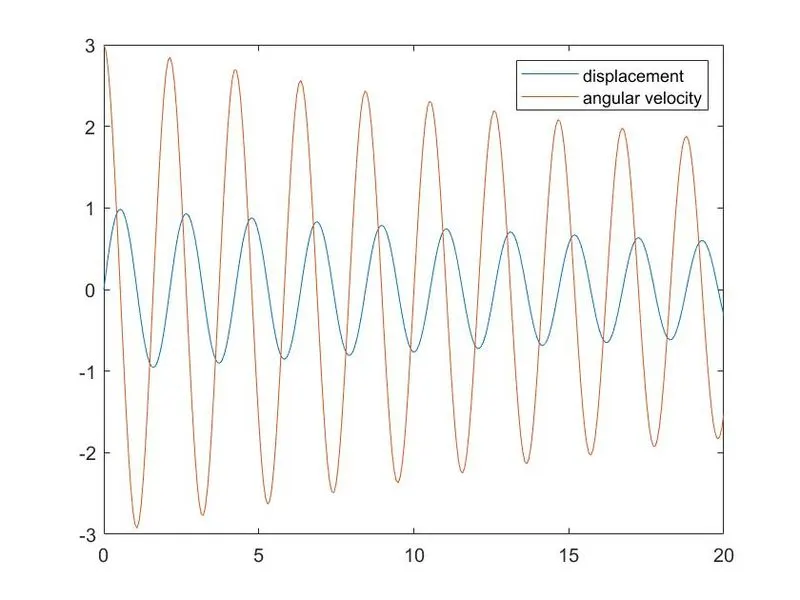
after solving the function we get results as an array of (300x2) which is displacement and angular velocity of 300 iteration

and we plot the displacement and angular velocity with respect to the time span

% For animating the motion of pendulum
figure(2)
ct=1
for i=1:length(results(:,1))
x0=0;
y0=0

x1=l*sin(results(i,1));
y1=-l*cos(results(i,1));

plot([0 0],[-1.5 0.5])
hold on
plot([x0 x1],[y0,y1],'LineWidth',1,'Color','b')
axis([-1.5 1.5 -1.5 0.5])
plot(x1,y1,'o','MarkerSize',20,'Color','r')
pause(0.0001)
M(ct)=getframe(gcf)
hold off
ct=ct+1
end

To create the animation of simple pendulum, we created the for loop to create the specified different points of bob position

x0, y0 is the fixed position of and x1, y1 is a different position of bob. 'ct' command which is used to count each and every position and stores the data

and at end of loop new set of position for each and every point

%making a video file
movie(M)
videofile=VideoWriter('simple_pendulum.avi','Uncompressed AVI')
open(videofile)
writeVideo(videofile,M)
close(videofile)

Here we use videowrite file is used to create the video file

The plot of displacement and angular velocity with respect to time

Link for a youtube video : https://www.youtube.com/watch?v=vxQ-CX0W4Vc