Week 4.1 - Genetic Algorithm

AIM: To write a code in MATLAB to optimize the stalagmite function and find the global maxima of the function

Theory:

First, we have to understand what is the optimization and how it works

Optimization: It is the process to find out the best results for a set of prioritized constraints and criteria

eg optimize length x width x height of a beam in such a way its FOS, stress, matrial consumed under some load is within the limit

Genetic algorithm is one of the optimization processes

What is a genetic algorithm?

A genetic algorithm (GA) is a method for solving both constrained and unconstrained optimization problems based on a natural selection process that mimics biological evolution.

It follows the following process

• Initialization: Initializing population which is a sample data points taken to perform genetic algorithm
• Selection: Selecting parents from the population-based on their fitness score (higher the fitness score higher the probability to be selected as a parent
• cross-over: it is the process of taking two parents and producing a child(new output) from them by interchanging the genes
• Mutation: It is done to maintain the genetic diversity of one generation of the population to another, if mutation is not performed output sample space will become similar and results in local minima

GA Syntax

clear all
close all
clc
x= linspace(0,0.6,150);
y= linspace(0,0.6,150);
num_cases=50;
[xx yy]= meshgrid(x,y);
for i=1:length(xx)
    for j=1:length(yy)
        input_vector(1)=xx(i,j);
        input_vector(2)=yy(i,j);
        f(i,j)= stalagmite(input_vector);
    end
    
end
surfc(xx,yy,f)
xlabel('xvalue')
ylabel('yvalue')

tic
% study1- unbounded conditions
for i=1:num_cases
    [inputs,fopt(i)]=ga(@stalagmite,2);
    xopt(i)=inputs(1);
    yopt(i)=inputs(2);
end
study1_time=toc
figure(1)
subplot(2,1,1)
hold on
surfc(x,y,-f)
shading interp
plot3(xopt,yopt,-fopt,'marker','o','markersize',5,'MarkerFaceColor','r')
title('unbounded inputs')
subplot(2,1,2)
plot(-fopt)
xlabel('Iterations')
ylabel('function minimum')

tic
%study 2- stastical behaviour-with upper and lower bound
for i=1:num_cases
   [inputs,fopt(i)]=ga(@stalagmite,2,[],[],[],[],[0;0],[1;1]);
    xopt(i)=inputs(1);
    yopt(i)=inputs(2);
end
study2_time= toc;
figure(2)
subplot(2,1,1)
hold on
surfc(x,y,-f)
shading interp
plot3(xopt,yopt,-fopt,'marker','o','markersize',5,'MarkerFaceColor','r')
title('bounded inputs')
subplot(2,1,2)
plot(-fopt)
xlabel('Iterations')
ylabel('function minimum')

% study 3 - Increasing ga iterations
options= optimoptions('ga')
options= optimoptions(options,'PopulationSize',300);

tic
for i=1:num_cases
   [inputs,fopt(i)]=ga(@stalagmite,2,[],[],[],[],[0;0],[1;1],[],[],options);
    xopt(i)=inputs(1);
    yopt(i)=inputs(2);
end
study3_time= toc;
figure(3)
subplot(2,1,1)
hold on
surfc(x,y,-f)
shading interp
plot3(xopt,yopt,-fopt,'marker','o','markersize',5,'MarkerFaceColor','r')
title('bounded inputs with modified population size')
subplot(2,1,2)
plot(-fopt)
xlabel('Iterations')
ylabel('function minimum')

Stalagmite function program :

function f= stalagmite(input_vector)
x=input_vector(1);
y=input_vector(2);

f1= (sin(5.1*pi*x+0.5))^6;
f2= (sin(5.1*pi*y+0.5))^6;
f3= exp((-4*log(2)*(x-0.0667)^2)/0.64);
f4= exp((-4*log(2)*(y-0.0667)^2)/0.64);

f= -(f1*f2*f3*f4);
end

Code explanation:

clear all
close all
clc
x= linspace(0,0.6,150);
y= linspace(0,0.6,150);
num_cases=50;

First, we initialize values of x and y by 150 values between 0 to 0.6, considering 50 iteration num_cases.

[xx yy]= meshgrid(x,y);
for i=1:length(xx)
for j=1:length(yy)
input_vector(1)=xx(i,j);
input_vector(2)=yy(i,j);
f(i,j)= stalagmite(input_vector);
end

Here we form 2d array by using meshgrid command and saving them as input for the stalagmite function, here we use 'for loop' to get the 'f' value over the length of x and y

we write stalagmite function according to its formula and we have taken 'f' output as '-ve' sign becuase 'ga' only minimise the function so taking '-ve' f will get us maxima

tic
% study1- unbounded conditions
for i=1:num_cases
[inputs,fopt(i)]=ga(@stalagmite,2);
xopt(i)=inputs(1);
yopt(i)=inputs(2);
end
study1_time=toc
figure(1)
subplot(2,1,1)
hold on
surfc(x,y,-f)
shading interp
plot3(xopt,yopt,-fopt,'marker','o','markersize',5,'MarkerFaceColor','r')
title('unbounded inputs')
subplot(2,1,2)
plot(-fopt)
xlabel('Iterations')
ylabel('function minimum')

First study: first we have taken a number of iterations to num_cases, we use a genetic algorithm to calculate the maxima function and store output as values at which maxima are obtained here we stored inputs and 'xopt' 'yopt'. plot surface of x,y,-f and use plot 3 commands for plotting xopt,yopt,-fopt for optimum maximas. also plotting 'fopt' to see optimum values at each iteration

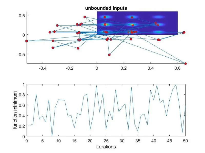
Here we can see optimum values are outside of x and y so located outside of stalagmite surface most of the time,here we can not reach global maxima

study time=2.7235

study 2 with bounded outputs

tic
%study 2- stastical behaviour-with upper and lower bound
for i=1:num_cases
[inputs,fopt(i)]=ga(@stalagmite,2,[],[],[],[],[0;0],[1;1]);
xopt(i)=inputs(1);
yopt(i)=inputs(2);
end
study2_time= toc;
figure(2)
subplot(2,1,1)
hold on
surfc(x,y,-f)
shading interp
plot3(xopt,yopt,-fopt,'marker','o','markersize',5,'MarkerFaceColor','r')
title('bounded inputs')
subplot(2,1,2)
plot(-fopt)
xlabel('Iterations')
ylabel('function minimum')

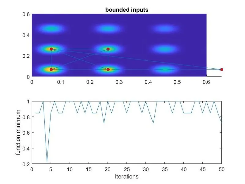
here we specify upper and lower bounds for x and y and followed same procedure as explained in previou study, we use tic and toc command to measure time taken for study

now optimum values are within limits but we can not achieve the global maxima value

study time: 5.14 sec

study 3 bounded values with an initial population

% study 3 - Increasing ga iterations
options= optimoptions('ga')
options= optimoptions(options,'PopulationSize',300);

tic
for i=1:num_cases
[inputs,fopt(i)]=ga(@stalagmite,2,[],[],[],[],[0;0],[1;1],[],[],options);
xopt(i)=inputs(1);
yopt(i)=inputs(2);
end
study3_time= toc;
figure(3)
subplot(2,1,1)
hold on
surfc(x,y,-f)
shading interp
plot3(xopt,yopt,-fopt,'marker','o','markersize',5,'MarkerFaceColor','r')
title('bounded inputs with modified population size')
subplot(2,1,2)
plot(-fopt)
xlabel('Iterations')
ylabel('function minimum')

Here we increase the initial population size from 50 to 300 and followed the same process as first two studies

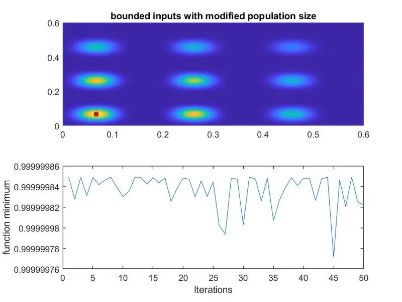
Here we find the correct maxima for the stalagmite function hence we can see that by increasing the initial size of the population we can increase the accuracy of ga

Errors occur while programming :

• I forgot to consider 'f' and -ve so ga minimizes the stalagmite function and i was getting wrong plots