Project
Carry out a system-level simulation of an all-terrain vehicle.
Download the model from the given link:
https://www.mathworks.com/matlabcentral/fileexchange/70576-baja-all-terrain-vehicle-atv-model
Prepare a technical report explaining the model properties & comments on the results.
Aim:
To study system-level simulation of an all-terrain vehicle and explain the results.
All-Terrain Vehicle:
An All-terrain vehicle (ATV), also known as a quad, three-wheeler, four-track, four-wheeler, or quadricycle, as defined by the American National Standards Institute (ANSI) is a vehicle that travels on low-pressure tires, with a seat that is straddled by the operator, along with handlebars for steering control. Suzuki was a leader in the development of mass production four-wheeled ATVs. It sold the first model, the 1982 Quad Runner LT125, which was a recreational machine for beginners.
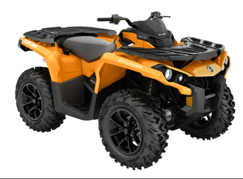
Safety has been a major issue with ATVs due to the high number of deaths and injuries associated with them and the negligible protection offered by the machine.
In ATV’s the rider sits on and operates these vehicles like a motor cycle, but the extra wheels give more stability at lower speeds. Although most are equipped with three or four wheels, six-wheel model exists for specialized applications. The Sport models are built with performance, rather than utility, in mind. To be successful at fast trail riding, an ATV must have light weight, high power, good suspension and a low centre of gravity.
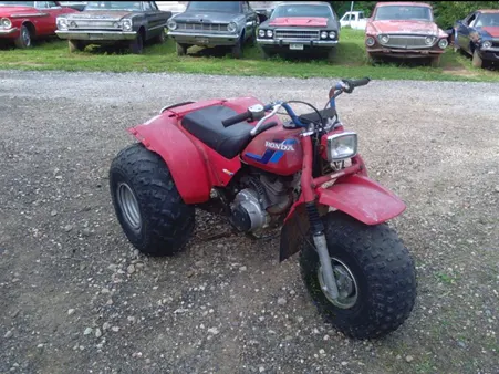 Three-wheel
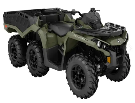
six-wheel
It is designed to handle a wider variety of terrain than most ither vehicles. ATVs come in many different shapes and sizes. The different types of ATVs are designed and manufactured for different uses including racing, pit-vehicles, recreation, hunting, ranching, military, emergency services, and industrial usage.
All-Terrain-Vehicle were making by 1. KS Ventures 2. Cryptic Adventure Sports Private Limited 3. Balaji Adventure 4. Amir Traders 5. Avery Freewheel Pvt. 6. Uboard India Limited 7. Haris Traders 8. ANIS TEXTILES 9. Humz Collection 10. Acriolis India Motors Private Limited and etc in india.
The Simulink model of the ATV is,
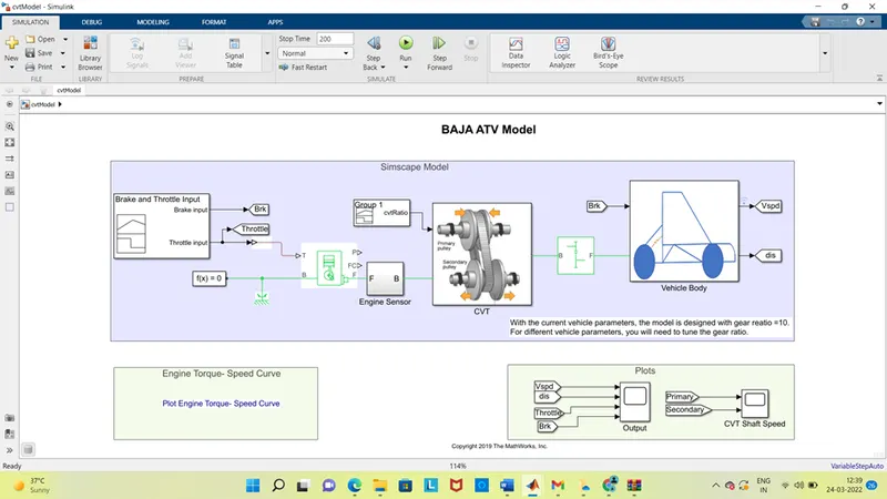
The model that we are seeing is the BAJA ATV model. In this the major components are,
- Continuously variable Transmission (CVT)
- Vehicle body
- Generic engine
- Simple gear
- Tires and breaks
Continuously variable Transmission
A continuously variable transmission (CVT), also known as a shiftless transmission, stepless transmission, pulley transmission is an automatic transmission that can change seamlessly through a continuous range of effective gear ratios. This contrast with other transmissions that provide a limited no of ger ratios in fixed steps. The CVT Controller block implements a push belt continuously variable transmission CVT controller. The block uses standard pulley and geometric equations to calculate the kinematic setpoints for the CVT variator. You can use the block to control a CVT. It is a system, that changes gear ratio with a change in the input RPM and the torque feedback at the wheels. The CVT does not strictly require the presence of a clutch. Nevertheless, in some cases, a centrifugal clutch is added to facilitate a “neutral” stance, which is useful when idling or manually reversing. A belt-driven design offers approximately 88% efficiency.
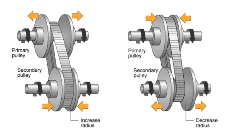
Here the low gears can provide a better acceleration while higher gears can maximize fuel economy. CVTs are different from traditional automatic transmissions in that they don’t have the gears that provides steps between low and high-speed operations. Instead of that the majority of them work via a pair of variables- diameter, cone-shaped pulleys connected by a steal or composition belt.
To run the model in practical In this way, the model design of the CVT is look like as shown,
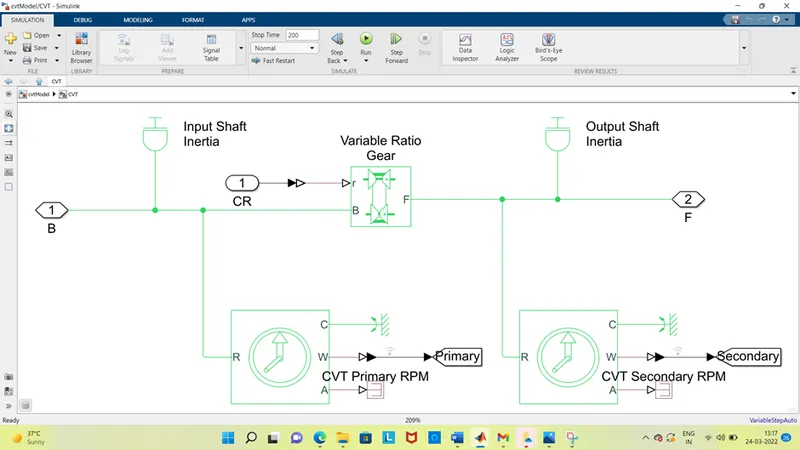
As we observe here that the CVT block sub system contains variable gear ratio, input and output shaft inertia, CVT primary and secondary rpm sensors with scopes. The scopes are used to see the results as a graphical path.
Variable gear ratio:
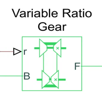
This example shows a variable ratio gear coupling two inertias (shafts). The gear ratio between the follower (F) and the base (B) is steadily increased from 1:1 to 2:1.
The physical signal input ‘r’ defines the ratio of input and output angular shaft velocities. The ratio of the follower to base angular speed decreases with gear ratio, and follower to base torque increases with gear ratio respectively. The variable gear is implemented using the Variable Ratio Transmission block which includes compliance. Appropriate stiffness and damping values for the compliance will depend upon the levels of torque transmitted by the variable gear. If the compliance damping is unrealistically low, the system can develop high frequency oscillations that require small simulation time steps.
VEHICLE BODY:
The vehicle body is look like this.
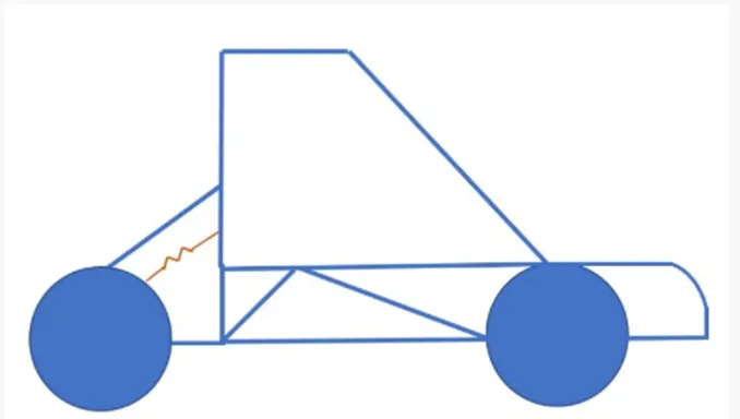
The vehicle body sub-system includes vehicle body block, double drum brake, and tires, wind velocity, inertia and some other blocks as shown in below.
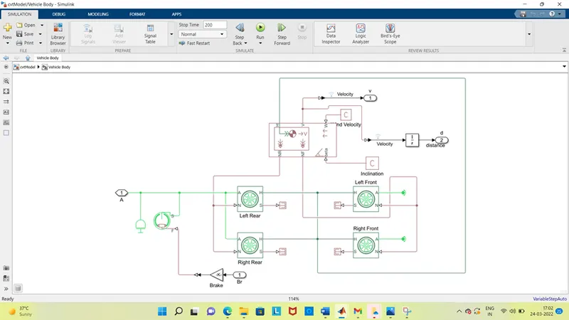
The vehicle body is used to represent the vehicle in practical way it has the same inputs as a real-world vehicle requires like drag values, pitch, variables.
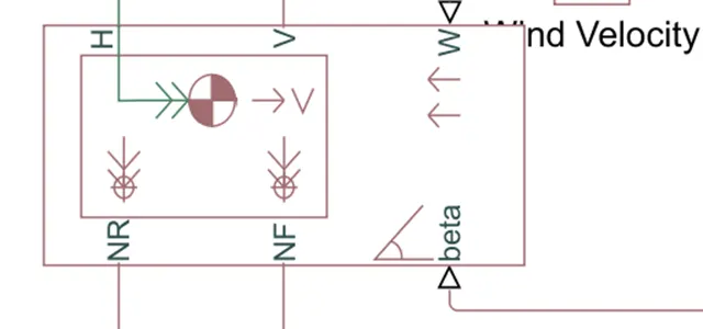
Vehicle body block.
This block has an option to include an externally-defined mass and an externally-defined inertia. The mass, inertia, and centre of gravity of the vehicle body can vary over the course of simulation in response to system changes.
The parameters in the vehicle body block are,
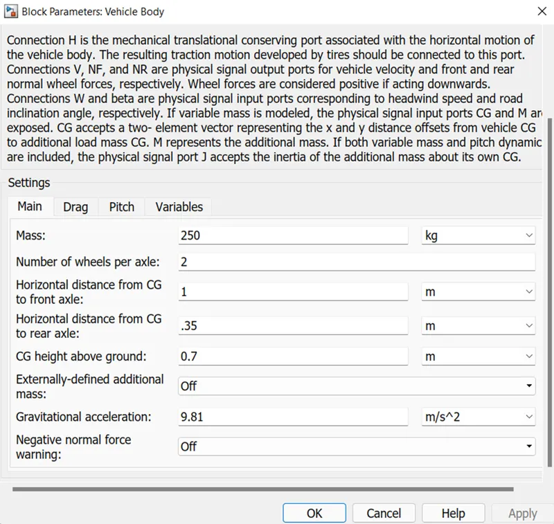
Mass of the vehicle = 250 kg
Front and rear axle with 4 wheels, we use two per axel as mentioned
We can change the parameters as our requirement, but place the standard values as same.
As the same the other parameters like tire block as shown below,
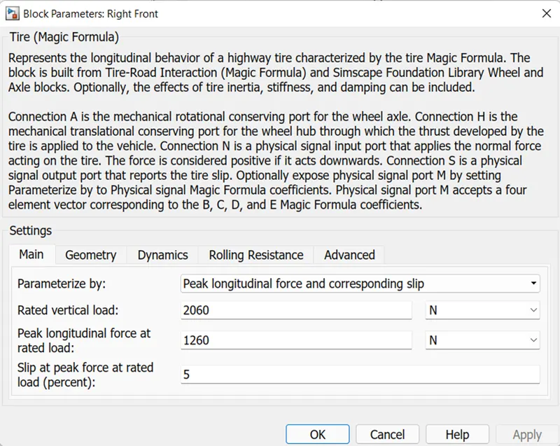
it also having some parameters that which have to be in as same as given.
In the sub system the output of the vehicle body block v is used to find the velocity and the integration of the velocity gives the distance of the vehicle travelled.
Generic engine:
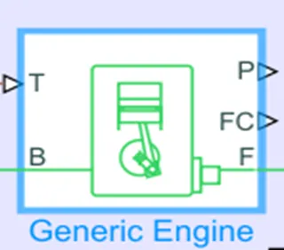
The generic engine block is a block which is located in Simscape / Driveline / Engines. It is used to represents a general internal combustion engine (IC) which is have two types those are compression ignition (CI-diesel) and spark ignition (SI-petrol).
In the block the values F and B are mechanical rotational conserving ports associated with the engine crankshaft and engine block, respectively. And the P and FC are physical signal output ports through which engine power and fuel consumption rate are reported. T is the Physical signal input port specifying the normalized engine throttle level. This Port T accepts a signal with values in the range 0–1
The parameters of the generic engine are look like as shown below.
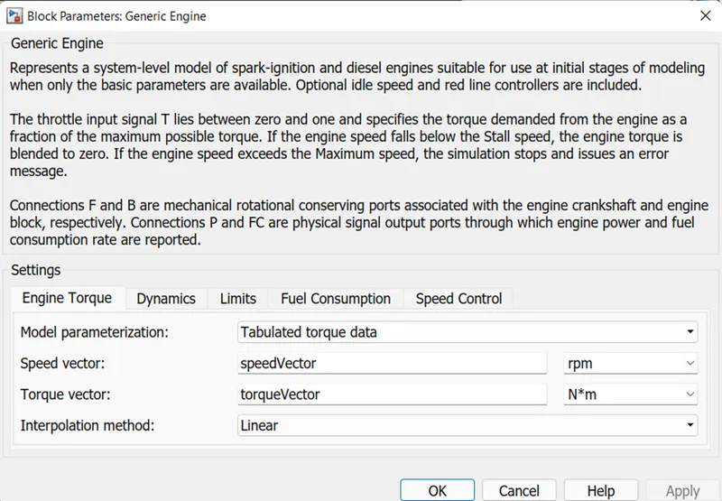
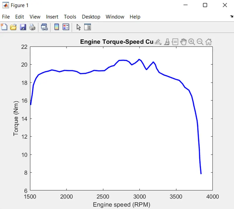
The parameters speed vector and the torque vector are here taken from the graph Engine Torque-Speed Curve from the model which is be plotted with specific values as shown below.
Simple gear:
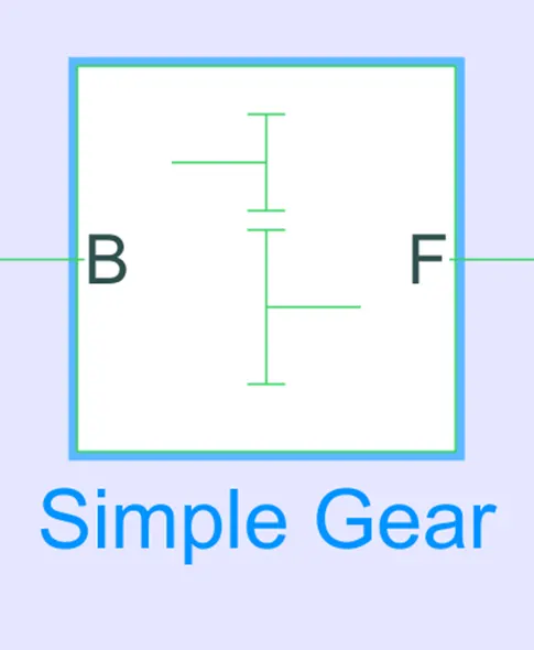
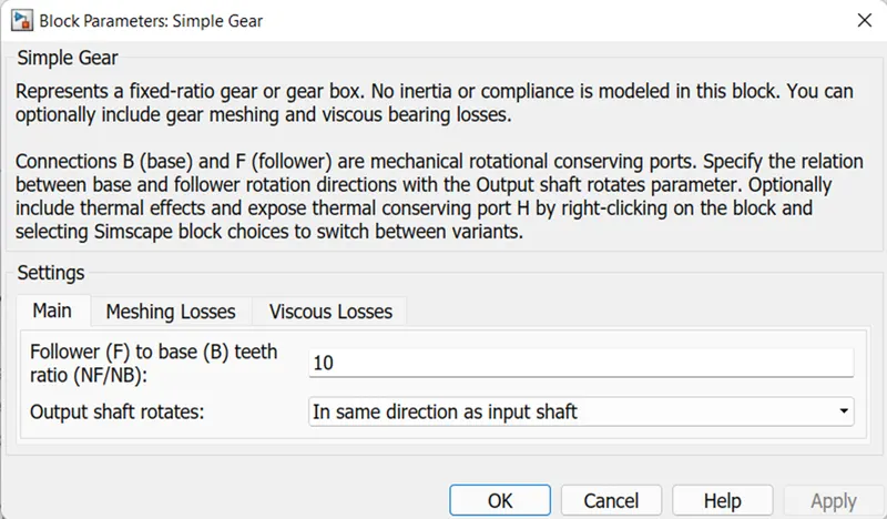
The simple gear is a block which is used to connect two inertias that is shafts. Simple gear of base and follower wheels with adjustable gear ratio, friction losses, and triggered faults. This block Represents a fixed-ratio gear or gear box. No inertia or compliance is modelled in this block. You can optionally include gear meshing and viscous bearing losses.
In the simple gear block the simple gear is a combination of a driver and driven gear where the speed is reduced by the gear ratio. It represents a gearbox that constrains the connected driveline axes of the base gear, B, and the follower gear, F, to corotate with a fixed ratio that you specify. You choose whether the follower axis rotates in the same or opposite direction as the base axis. If they rotate in the same direction, the angular velocity of the follower, ωF, and the angular velocity of the base, ωB, have the same sign. If they rotate in opposite directions, ωF and ωB have opposite signs. You can easily add and remove backlash, faults, and thermal effects.
The parameters of the simple gear block is show below,
Tires and breaks:
As we seen above that the tires are used in the vehicle body which is having the 2 tires each per axle which moves along with the given throttle value. It is the mathematical model of the design or block of the tire which have the same parameters and effects which are designed In the model as real.
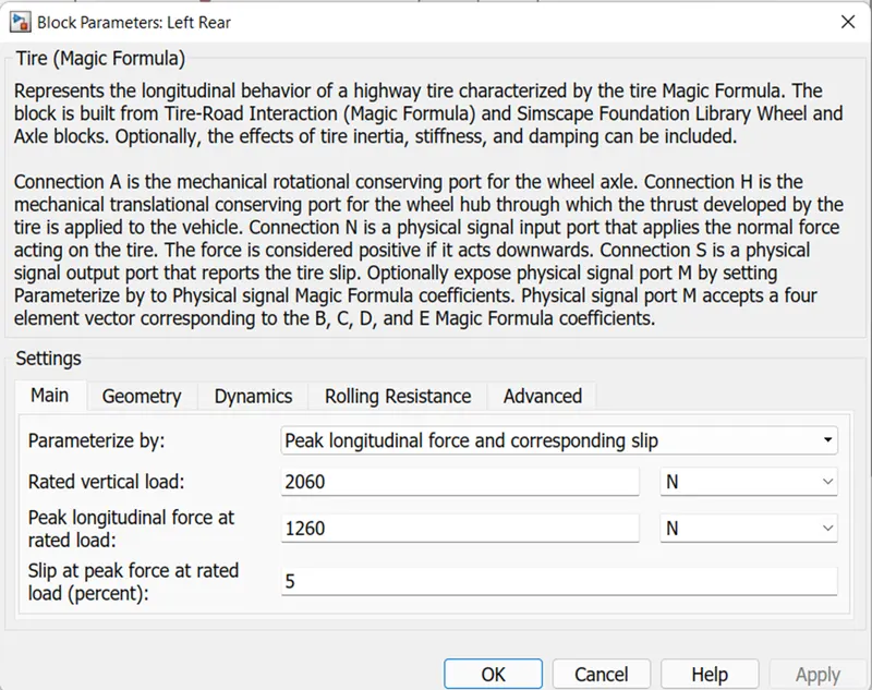
The values used in the above represents and gives the exact real tire values. It does not require any input like throttle values to run it runs as per the axel runs.
The brake system, the breaks is the given input value that can already derived by the signal builder with a specific value. If the given values is 1 then the break is applied to it otherwise it be in normal position.
The Double-Shoe Brake block represents a frictional brake with two pivoted rigid shoes that press against a rotating drum to produce a braking action. The rigid shoes sit inside or outside the rotating drum in a diametrically opposed configuration. A positive actuating force causes the rigid shoes to press against the rotating drum. Viscous and contact friction between the drum and the rigid shoe surfaces cause the rotating drum to decelerate it also have some measured values which will have to be in standard values.
The model taken for the study is the BAJA ATV model with Continuously Variable Transmission (CVT).
Explanation: by this model we are studying the BAJA ATV model by using the CVT.
There are different types of models those are,
- BAJA ATV model without dashboard
- BAJA ATV model with dashboard
- BAJA ATV model using the lookup table without a dashboard
- BAJA ATV model using the lookup table with a dashboard
Among all we will study about the BAJA ATV model with dashboard:
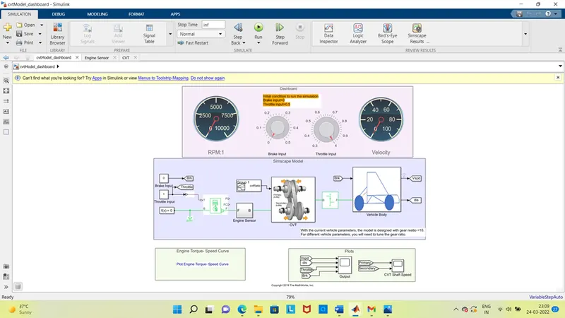
The study is based on ‘Baja ATV with dashboard’ as shown in the figure above here the input data like throttle and brake input are given from the dashboard instead of using a signal builder. All the remaining blocks are the same as in study above
The main intention behind the usage of the dashboard is to study the output value with the variation in throttle and brake which we can change as a real output, which will give the value of rpm and velocity of the engine in the digital reading.
Here as it mentions that at starting the values is be placed in given condition that is break input is ‘0’ and the throttle input is ‘0.5’.
Case 1:
Now if we run the model for 100 sec then the output values are plotted as shown below.
The first plotted results is the Engine Torque-Speed curve characteristics.
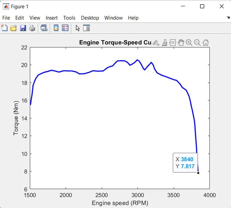
In the above plot Maximum Velocity reaches at 3840 RPM, and the Vehicle Speed is depending on CVT Ratio input values.
By keeping these values, we got the plot output scope one is the,
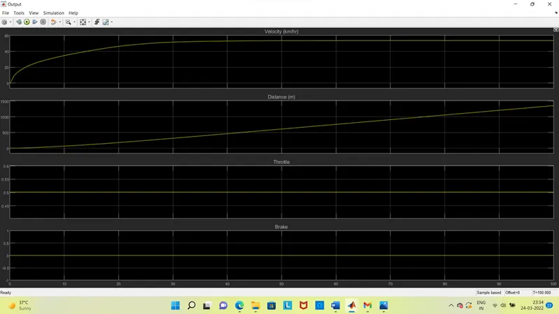
In this graph we got the results for the given input values, throttle and break input as 0.5 and 0 respectively. By these inputs we got the output values are the velocity (Km/Hr) and the distance in meters (m) with respect to time (T). as we observe that in the velocity one the speed moves to 52 kmph from 0 within 25 sec nearly and placed as constant up to 100, that is it takes very less time to reach high speed by giving less throttle input due to its motor speed range.
As the same when we observe that the distance results it changed maximum linearly up to 1343 meters in 100 sec.
From the second plot that is from the CVT Shaft Speed scope we can observe the results as below,
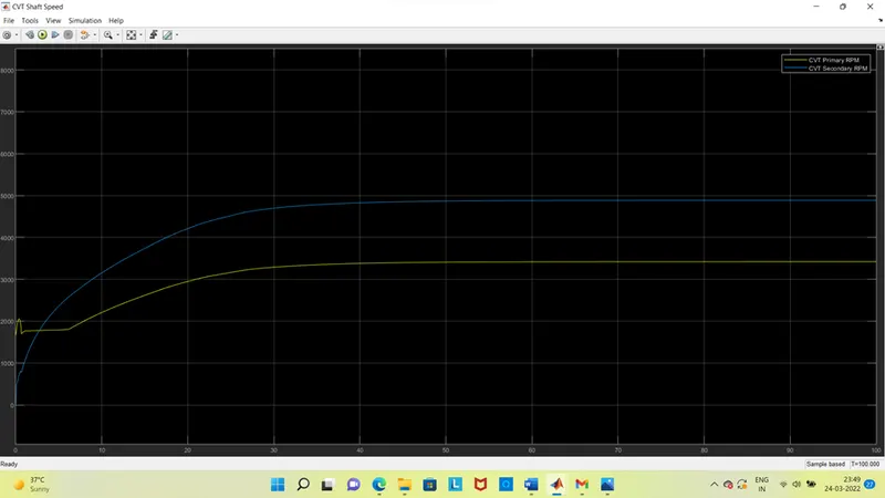
from these observations we can say that is an over drive type which CVTs of Primary Pulley goes inward and Secondary Pulley goes Outwards it will lead to Overdrive. Primary Pulley radius increases and Secondary Pulley radius decreases so Speed of Primary pulley is greater than Secondary Pulley so that its primary rpm is less than secondary rpm.
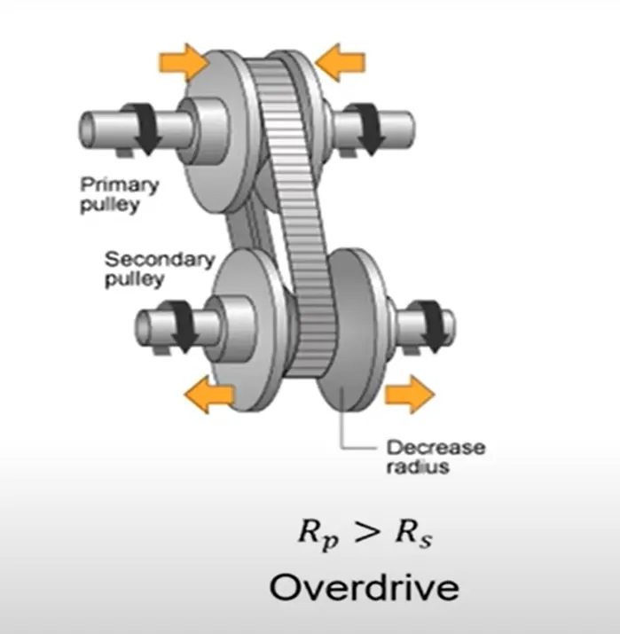
So as per the above Plot, Brake Input is 0 and Throttle input is 0.5 for 100 sec Engine Speed will decrease at the beginning because of increasing gear ratio which increases the torque and by increasing the Throttle input value to 0.5, then Engine Speed value will decrease because of increasing gear ratio and it reaches the maximum speed that is 3840 rpm speed.
By all these observations we can say that the by changing the values of the inputs in the dashboard model based on user point of view in every sec and we can plot each value and observe the results based on the given input values.
Case 2:
Now if we observe the break values and also the changes in the throttle input values in 100 sec we got the results as,
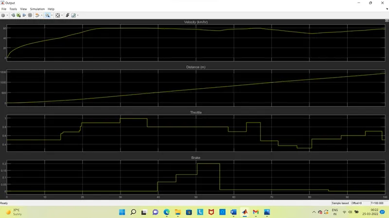
From this output result graph, we can see how we changed the throttle input value and the break input value by these changes we observe the output of the distance and velocity respectively. As we observe that the distance is placed as near to previous value but the velocity changes are very fluctuated due to no of changings in the throttle value.
If we observe the CVT Shaft Speed scope results we get the values as,
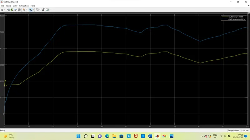
Here also at starting the values are started at same as previous one but after the changes in the throttle input and the break input values it places a fluctule changes in the CVT values but the secondary rpm is placed more than the primary RPM with the same distance range.
Case 3:
If we change the throttle by keeping the brake value 0.2 throughout the running the results is as shown below.
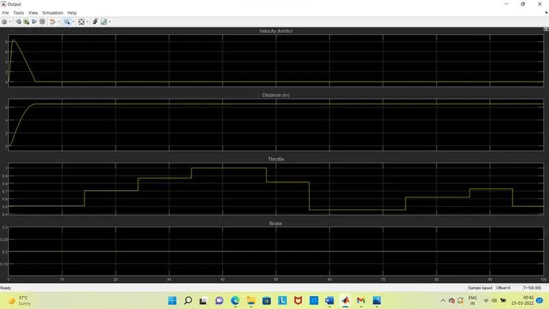
By this output results scope we can say that by keeping the break input with some value, if we change the throttle value to any value, we can’t change the velocity from zero. If we observe at the staring due it throttles 0.5 value its place some value up to 5 sec after that it attain to 0. As the same if we observe the distance value it reaches to some value 5 meters and it placed constant till the end even though there is change in the throttle.
As the same if we see the CVT Shaft Speed scope results we get the values as below,
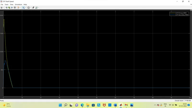
Here if we observe that the primary is placed at the top at starting it reaches to zero ‘0’ and remains constant till the end.
from these observations we can say that is an over drive type which CVTs of Primary Pulley goes outward and Secondary Pulley goes inwards it will lead to slow drive. And the Primary Pulley radius decreases and Secondary Pulley radius increases so Speed of Primary pulley is lower than Secondary Pulley so that its primary rpm is greater than secondary rpm.
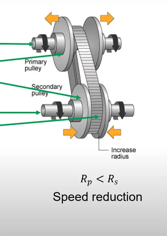
As the same from Engine Speed value will increase at beginning because of decreasing gear ratio which decrease the torque and it reaches the maximum speed that is 3840 rpm speed.
Like the same each model can calculate the model output values through input one in the different types like with dashboard, without dashboard by the look up table or without look up table by their results we can identify the values and characteristics of the all-terrain vehicle design model.
Conclusion:
By this all-terrain vehicle model design, we studied the simulation model type and how it be designed what are the results that we can observe while running. And also learn the model properties and its results of different models.