Project

ATV:-

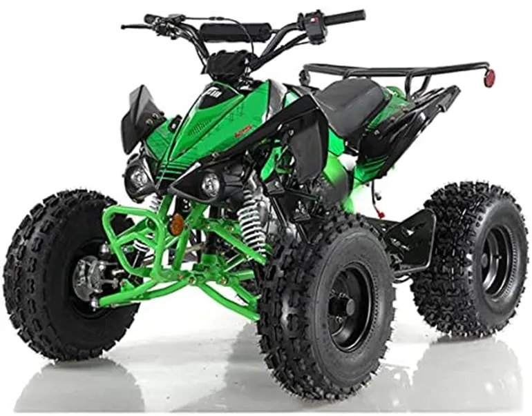
An all-terrain vehicle (ATV), also known as a light utility vehicle (LUV), a quad bike, or simply a quad, as defined by the American National Standards Institute (ANSI); is a vehicle that travels on low-pressure tires, with a seat that is straddled by the operator, along with handlebars for steering control. As the name implies, it is designed to handle a wider variety of terrain than most other vehicles. Although it is a street-legal vehicle in some countries, it is not street-legal within most states, territories and provinces of Australia, the United States or Canada.

By the current ANSI definition, ATVs are intended for use by a single operator, although some companies have developed ATVs intended for use by the operator and one passenger. These ATVs are referred to as tandem ATVs.

CVT:-

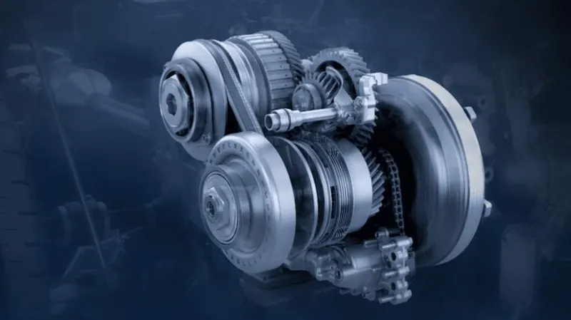
A continuously variable transmission (CVT) is an automatic transmission that can change seamlessly through a continuous range of gear ratios. This contrasts with other transmissions that provide a limited number of gear ratios in fixed steps. The flexibility of a CVT with suitable control may allow the engine to operate at a constant RPM while the vehicle moves at varying speeds.

CVTs are used in automobiles, tractors, motor scooters, snowmobiles, bicycles and earthmoving equipment.

The most common type of CVT uses two pulleys connected by a belt or chain; however, several other designs have also been used at times

Blocks Used:-

1. Generic Engine-
2. Rotational motion Sensor
3. Variable Ratio Gear
4. Simple Gear
5. Vehicle body
6. Tire

Case 1:-

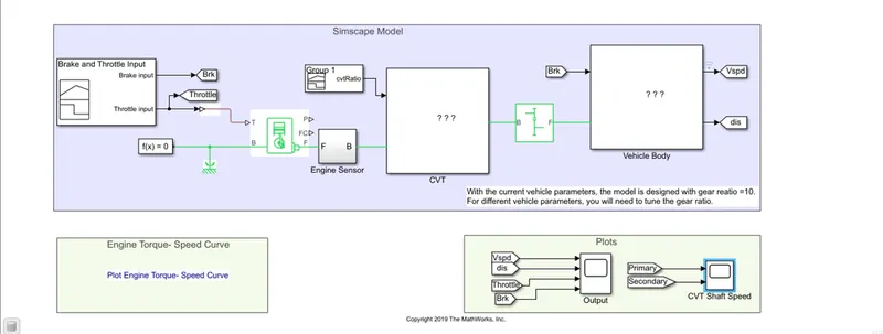
Figure (1)

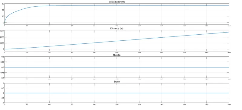
In this model a signal builder block is used to simulate the brake and throttle input. As seen from fig.(2), break input is 0 through out the simulation, while throttle input is 0.5.

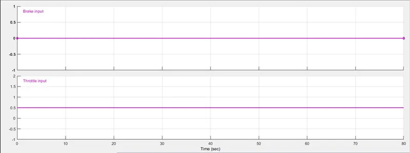
Figure (2)

The throttle input is given to a generic engine block. Various parameters like speed vector, torque vector, engine inertia, etc. can be entered in the generic engine block parameter settings. In this case only speed and torque vector parameters are entered. This parameters are extracted from a image of graph of BAJA engine speed-torque curve using one of the file exchangers ‘Grabit’ and then fed to the generic engine block.

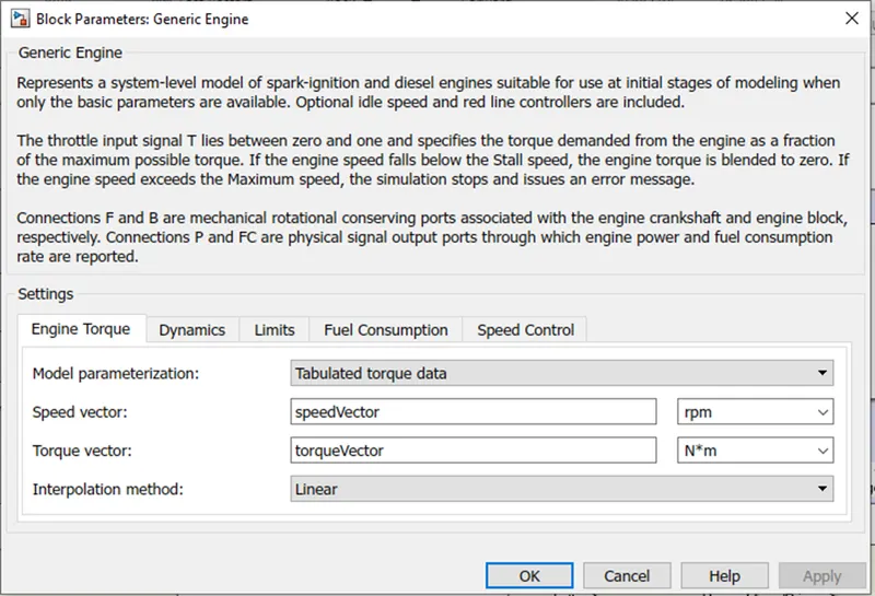
Figure (3)

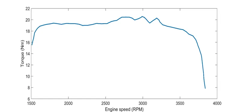
Figure (4)

An engine sensor is which is basically a rotational motion sensor is used to measure the engine RPM.

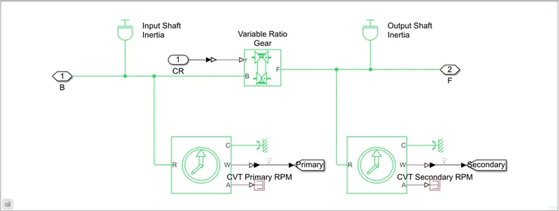
Figure (5)

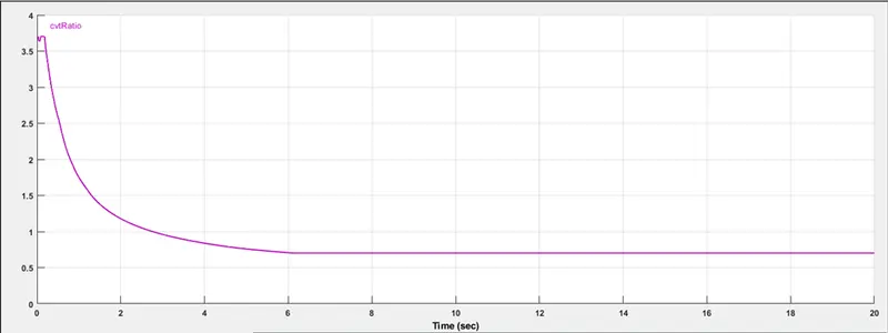
Figure (6)

The CVT sub-system has 2 inertia blocks- input shaft inertia and output shaft inertia. This 2 represents the input and output pulley inertia. There is also a variable ratio gear block to which gear ratio is provided by a signal builder block. As seen from fig(6) at start of the simulation the gear ratio is around 3.7 and then exponentially decreases to until the 6 seconds to a value of around 0.7 and then remains constant through out the simulation. Two rotational sensors are also used to measure the CVT primary RPM and CVT secondary RPM.

Figure(7)

The vehicle body subsystem has 4 tire blocks, one vehicle body block and one double shoe brake block. A simple gear ratio block is connected to the output of the CVT subsystem. In vehicle body subsystem the rotational output of the CVT system is connected to the rear wheel blocks. Break input from the signal builder 1 is given the double shoe brake block. The rated vertical load on all 4 wheels is 2060 N while rolling radius of rear wheels is 0.2921 m and that of front wheels is 0.267 m. The mass entered in the vehicle body block is 250 kg.

Figure(8)

Observation:-

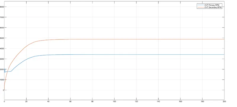
• As seen from fig(6) and (7) as CVT ratio decreases, the value of the CVT secondary RPM also exponentially increases.
• When the CVT ratio falls below 1 at the same time the CVT secondary RPM becomes more that CVT primary RPM. The CVT secondary RPM continuously increases exponentially till 40 seconds and then remains constant throughout the simulation.
• As observed from fig(8) the velocity also increases till 40 seconds and then remains constant.

Case 2:-

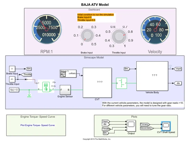
Figure (9)

The model for case 2 is similar to case with only difference is that the brake and throttle inputs are gives using a dashboard. Two knobs each for brake and throttle are connected to the constant blocks which fed the values in the model.

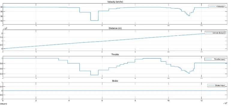
Figure (10)

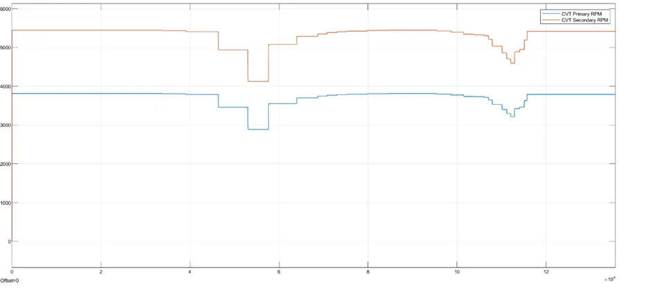
Figure (11)

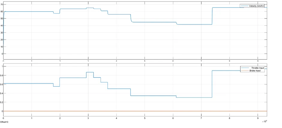
Fig (9) shows the relation between the throttle input the vehicle velocity. As observed from the fig(9)

The vehicle velocity varies with the knob position.

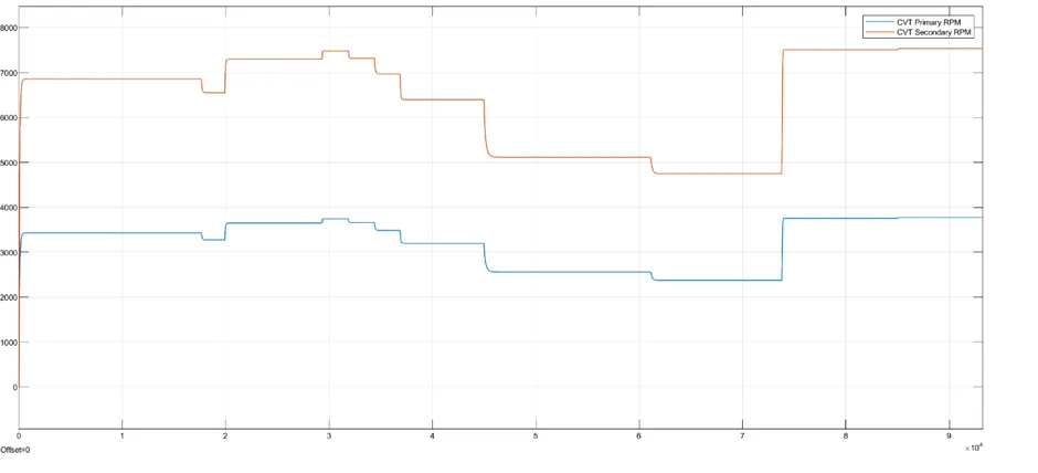
Similarly fig(11) shows the relation between the CVT primary RPM and CVT secondary RPM. It can be observed that the CVT secondary RPM varies similarly with the CVT primary RPM.

Case 3:-

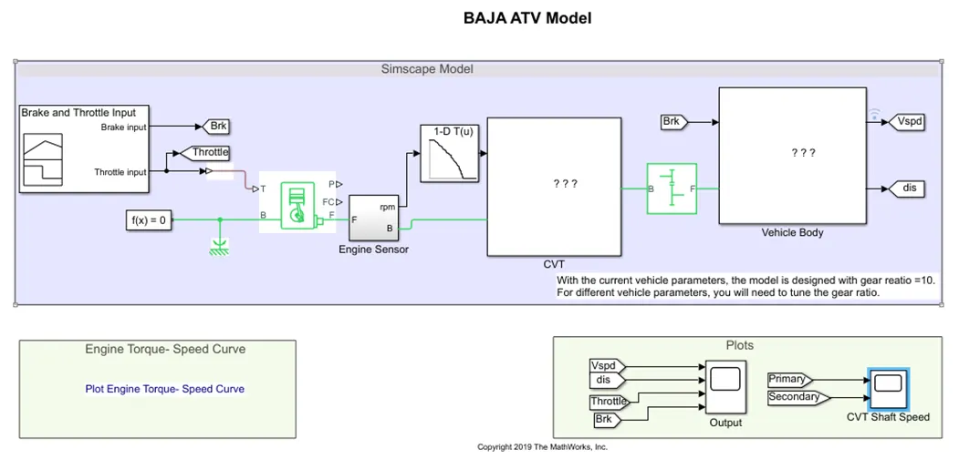
Figure(12)

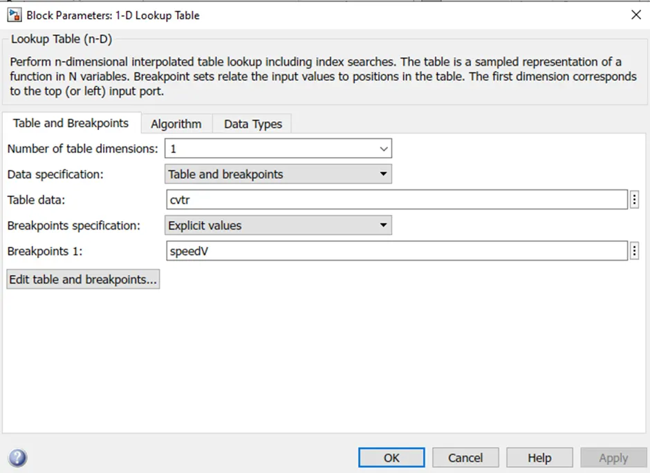
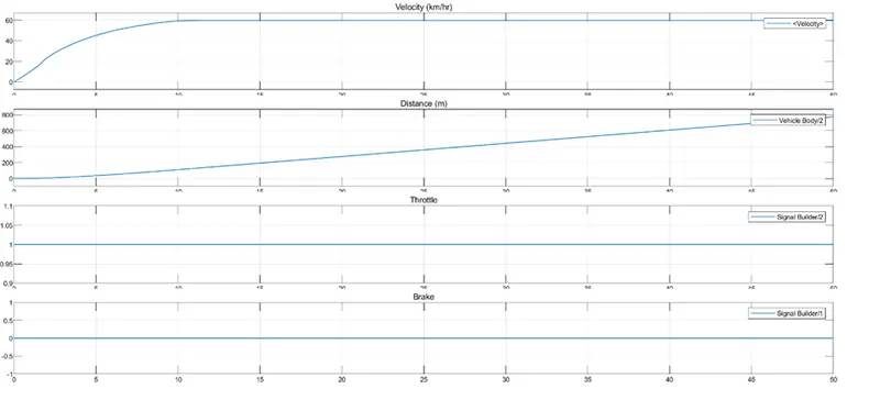
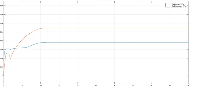
Fig(12) shows the Simulink model for BAJA ATV using lookup table. The difference here is that the variable ratio gear block from CVT system takes values of gear ratio from a 1-D look table. In a lookup table the pre-recorded or experimental data is put. In this case the data i.e. speed and CVT ratio is save in workspace as variables. The speed(RPM) values are put in ‘breakpoint 1’ and CVT ratio for respective speed is put in Table data as shown in fig(13). RPM input is taken from engine sensor block.

Figure(13)

Figure(14)

Figure(15)

Case 4:-

Figure(16)

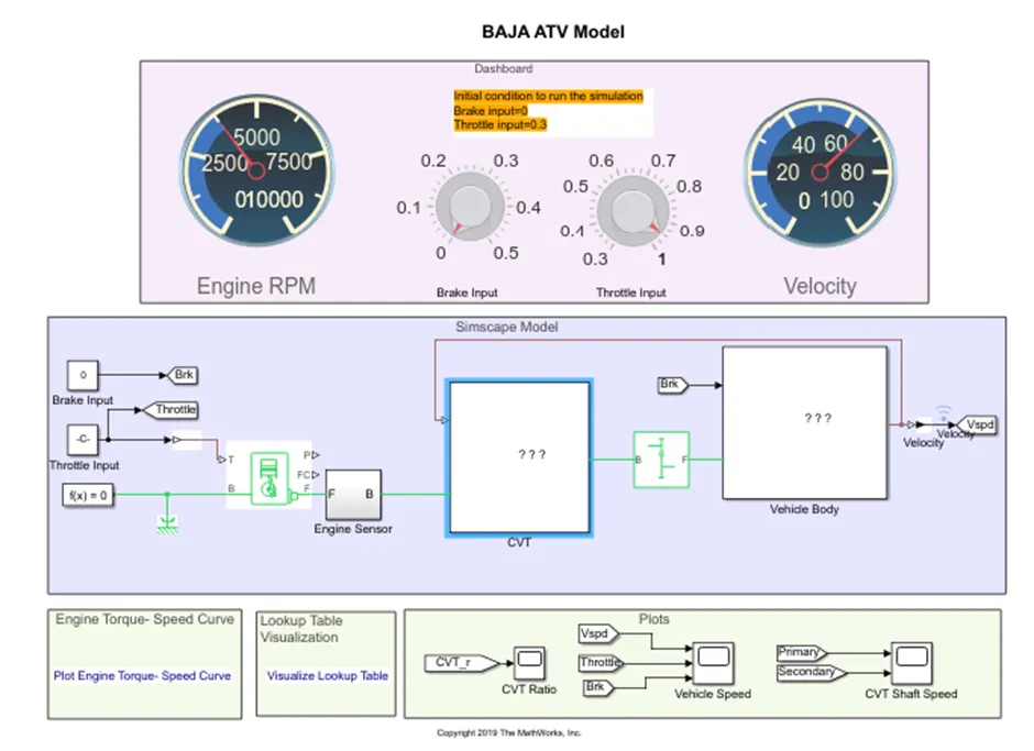
Fig(15) shows the simulink model for the BAJA ATV with dashboard and lookup table. This case is similar to the case 2 except the lookup table.

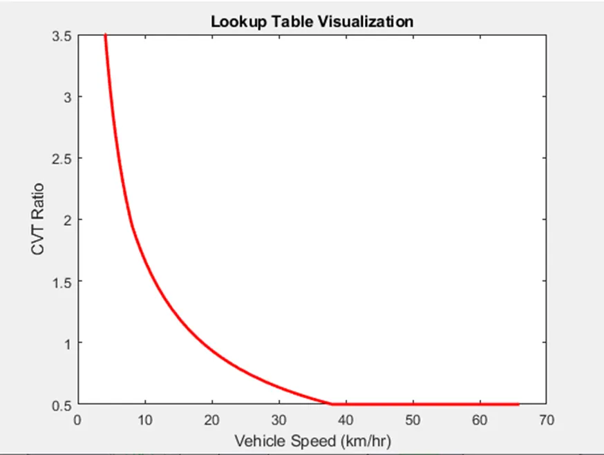
Figure(17)

In this case lookup table takes the vehicle velocity as the input and feds the respective CVT value to the variables ratio gear block. The CVT ratio at particular speed is derived from the graph shown in fig(16).

The throttle and brake input can be varied from the dashboard.