Project
AIM: To Carry out the system-level simulation of a terrain Vehicle using MATLAB simulink.
Objective: To Prepare a technical report on BAJA ATV explaining model properties and results for the following models.
Case1-BAJA ATV model without Dashboard.
Case2-BAJA ATV model with Dashboard.
Case3-BAJA ATV Model using Lookup table without Dashboard.
Case4-BAJA ATV model using Lookup table with Dashboard.
THEORY:
BAJA ATV: All Terrain Vehicle (ATV) is designed to run on different terrains or in other words we can say that ATV is specieally designed for Off roading conditions. The Vehicle consists of handle bars and low pressure tires that have deep threaded structures, which helps driving in muddy, rocky,wetlands etc. In comparison with other Utility vehicles (UTVs), ATVs offer excellent off road capabilities and can carry load over a long distances easily. they can also be customised for high performance riding, owing to which they find extensive applications across various industries including sports, entertainment , agriculture, military, defence etc. 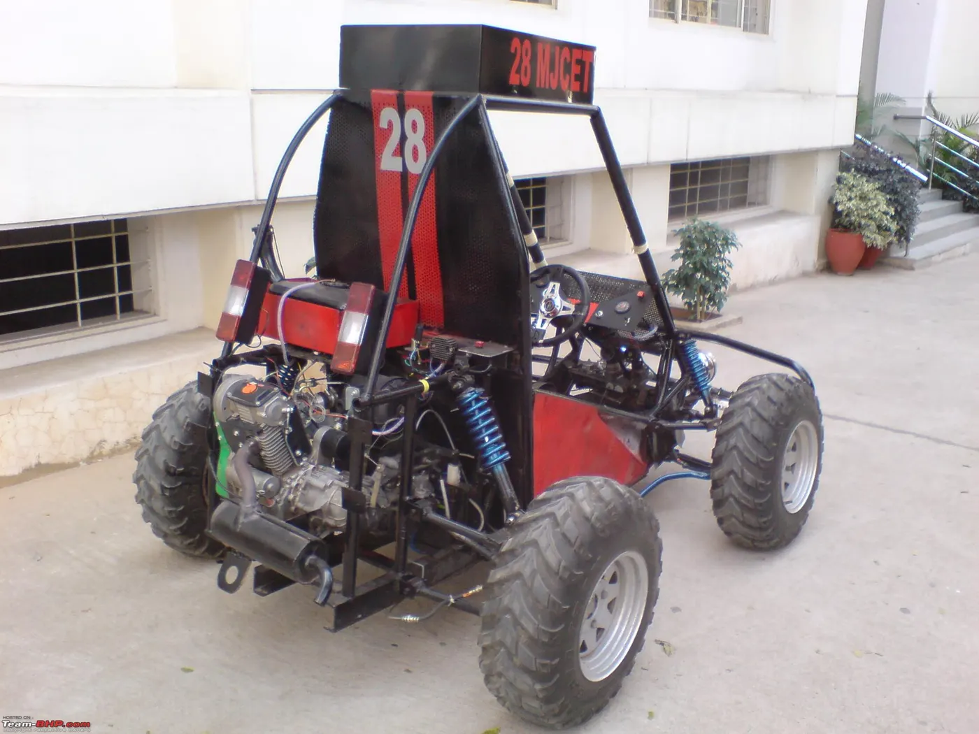
Major Blocks Used in the Simulation:
Generic Engine:
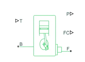
Represents a system-level model of spark-ignition and diesel engines suitable for use at initial stages of modeling when only the basic parameters are available. Optional idle speed and red line controllers are included. The throttle input signal T lies between zero and one and specifies the torque demanded from the engine as a fraction of the maximum possible torque. If the engine speed falls below the Stall speed, the engine torque is blended to zero. If the engine speed exceeds the Maximum speed, the simulation stops and issues an error message.
Ports:
F - mechanical rotational conserving ports associated with the engine crankshaft
B - mechanical rotational conserving ports associated with the engine block
P - physical signal output ports through which engine power is reported.
FC - physical signal output ports through which fuel consumption rate is reported.
Continous Variable Transmission (CVT):
CVT Consists of mainly Variable Diameter pulley, Driven pulley and belt or chain.
CVT is an automatic transmission system that can change seamlessly through a continous range of gear ratios. In comparision with other transmission systems that provide limited number of gear ratios in fixed steps. The flexibility of a CVT with suitable control may allow the engine to operate at a constant speed while the vehicle moves at variable speeds. CVTs are used in automobiles, tractors,motor cycles, snowmobiles etc.
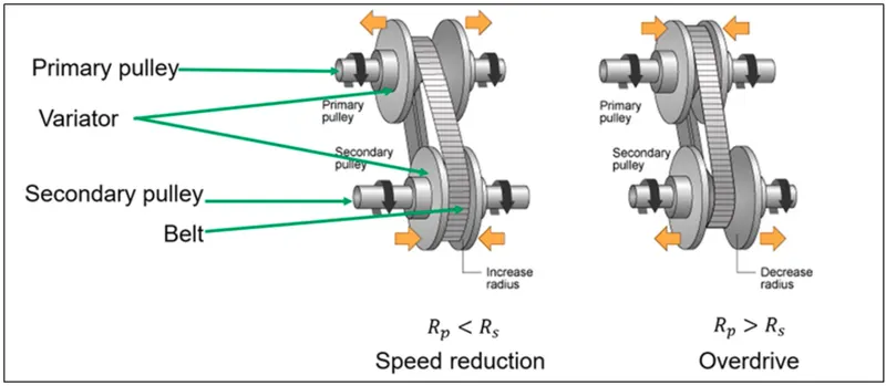
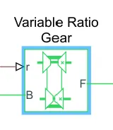
CVT replaces the gears with two variable diameter pulleys, each shaped like a pair of opposing cones with abelt or metal chain running between them.One pulley is connected to the engine shaft and the other to the drive wheels. the halves of the pulley are movable as the pulley halves come closer together the belt is forced to ride higher on the pulley, effectively making the pulley diameter larger. Changing the diameter of the pulley varies the transmission ratio. such that the primary or variable diameter pulley changes to large the secondary or driven pulley diameter will be smaller gives low gear ratio, which is better for low-speed acceleration. In the same way viceversa operation will be better for high-speed acceleration.
Ports:
r- Variable gear transmission input
B- Variable pulley input to CVT
F- Driven pulley output from CVT
Vehicle Body:
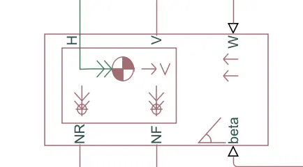
Represents a two-axle vehicle body in longitudinal motion. The block accounts for body mass, aerodynamic drag, road incline, and weight distribution between axles due to acceleration and road profile. The vehicle can have the same or a different number of wheels on each axle. Optionally include pitch and suspension dynamics or additional variable mass and inertia. The vehicle does not move vertically relative to the ground.
Ports:
H-the mechanical translational conserving port associated with the horizontal motion of the vehicle body
V- physical signal output port for vehicle velocity
w- physical signal input port to headwind speed
NR-physical signal output port for Rear Normal force
NF-physical signal output port for front Normal force
beta- physical signal input port to road inclination angle
Wheels:
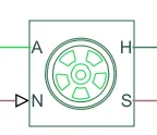
Vehicle body is connected to the four wheels of the vehicle body of two axles such that two tires are connected to one axle.
ports:
A- mechanical rotational conserving port for the wheel Axle
N-physical signal input port that applies the normal force acting on the tire
S-physical signal output port that reports the tire slip
H- mechanical translational conserving port for the wheel hub
Double Shoe Brake:
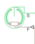
Represents a brake arranged as two pivoted rigid shoes symmetrically installed inside or outside a drum and operated by one actuator. The actuator force causes the shoes to exert a friction torque on a shaft connected to the drum.
Ports:
S- Conversing rotational terminal associated with the drum shaft
F-physical signal port representing the force input to the actuator
Blocks used for Simulation & purpose:
1. Signal Builder- To input the brake, throttle and CVT Ratio.
2. Simulink to PS coverter- To convertthe simulink signal to simscape environment
3. Solver configurtation: To specify solver parametres before starting the simulation.
4. Mechanical reference: for connecting the reference to ground for mechanical parameters.
5. Generic Engine: To run the engine with speed and tourque values as input.
6. PS-Simulink converter: To convert simscape signal to simulink environment
7. Scope: to plot the graphs of input and output signals
8. Display- to see the engine power
9. Inertia- To represent the solid inertia
10. Rotational motion sensor: To sense the rotational motion of engine and provides output as rpm.
11. VAriable gear ratio: To vary the speed by changine geaqr ratio
12. PS terminator: Terminator for for unconnected physical sinal outputs
13. Double shoe brake: To aplly brake to the vehicle when needed
14. PS- constant: generate constant physical signal
15. tire: for transportation of vehicle body
16. Vehicle body: to represent BAJA ATV model vehicle body
17. Custom Measure gauge- to read brake & throtle input
18. Knob: To vary the input signals for brake & throttle signals.
19. Lookup table: To insert CVT gear ratio values to workspace
20. Simple gear: To reduce or increase the speed of the wheels based on gear ratio
21. Step: To enable or disable the input value based on requirement
Simulnk models & Explaination:
Case:1 BAJA ATV model without Dashboard.
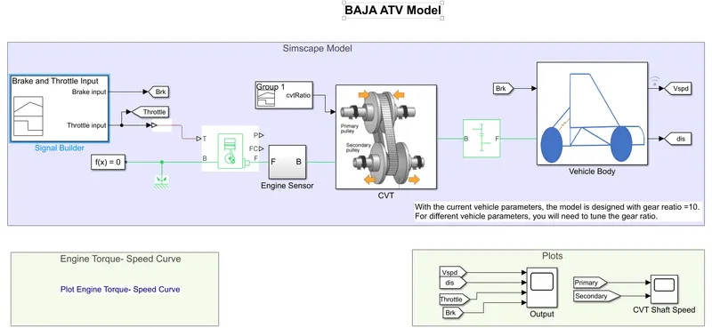
1. Using Signal builder two signals generated for brake and throttle input for generic engine. As generic engine is simscape block, needs a simulink to ps converter in between signal builder and generic engine. Speed threshold of generic engine is limited to 100 rpm and speed ,fuel controls are not selected.
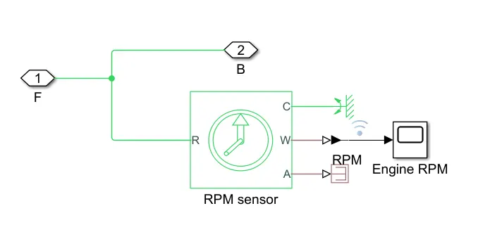
2. Generic engine output is connected to engine sensor to measure the speed of the engine shaft. then the engine output is connected to CVT input block.
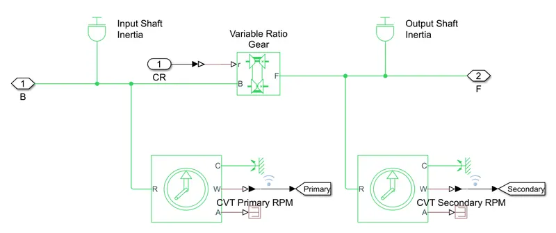
3. CVT subsystem created with input and output inertia block, Variable gear ratio and rotational motion sensor for input and output speed of CVT.
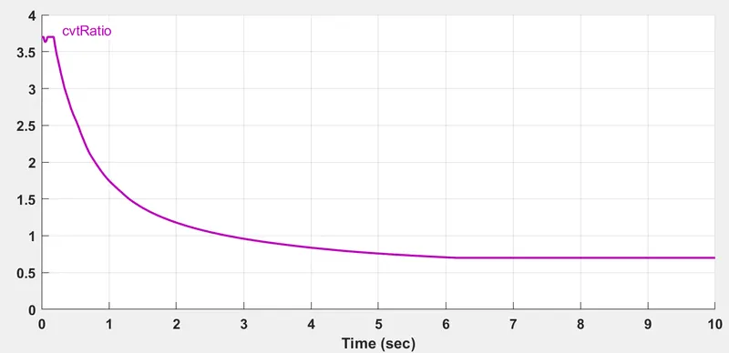
4. For CVT Gear ratio shall be given as a input to vary the gear ratio. In this model gear ratio changes are done by using signal builder as shown in graph.
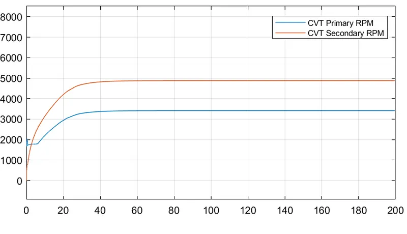
5. Based on the input to CVT (i.e., Cvt Gear ratio input) the gear ratio will be changing so that the acceleration at the shaft of secondary or driven pulley varies. The out put at port F is connected to the Simple gear block of port B. This simple gear system represents fixed gear ratio of 10 in this model.then the port F is connected to vehicle body. Vehicle body will be connected with wheel axles and tires with breakshoes to control the speed of vehicle during braek signal applies to it.
6. Speed of primary and secondary rpm of CVT is shoen below for the given input cvt signal.
Brake & throttle Input Signal to Generic engine Using signal builder:
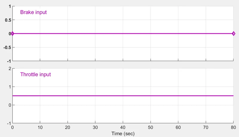
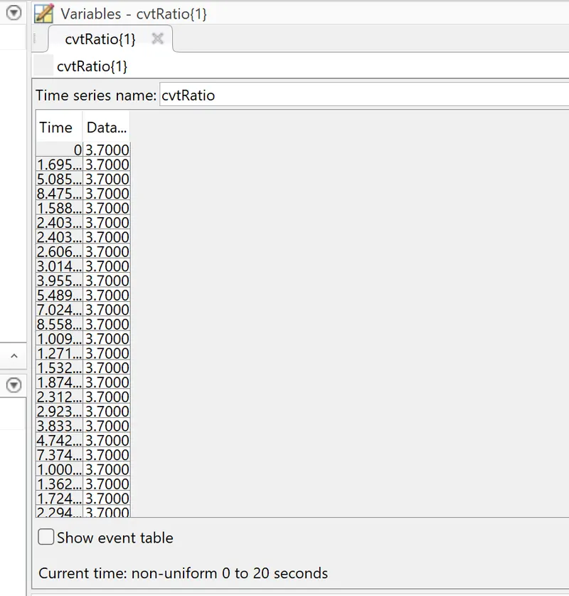
There is no brake input applied on the vehicle as the brake signal is constant at zero. Throttle input applied to the engine as 0.5 continously. And the cvt gear ratio is provided with respective time as shown below,
OUTPUT :
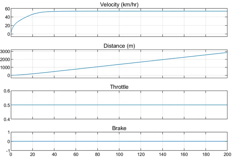
From the output graph we can observe that the velocity increases slowly and becoem constant from 40 sec thoughout the distance. since the no brakes are applied and throttle input is same as at 0.5.
Note: if we increase the throttle value fuel consumption will increase so that the engine acceleration also will increase).
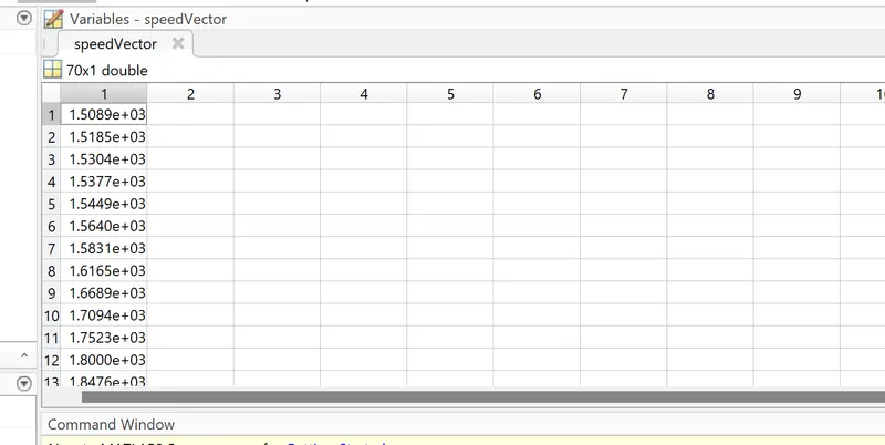
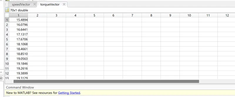
Speed vector and torque vector is saved in the workspace as shown below,
The Characterisitics of Speed vector vs torque vector is shown below
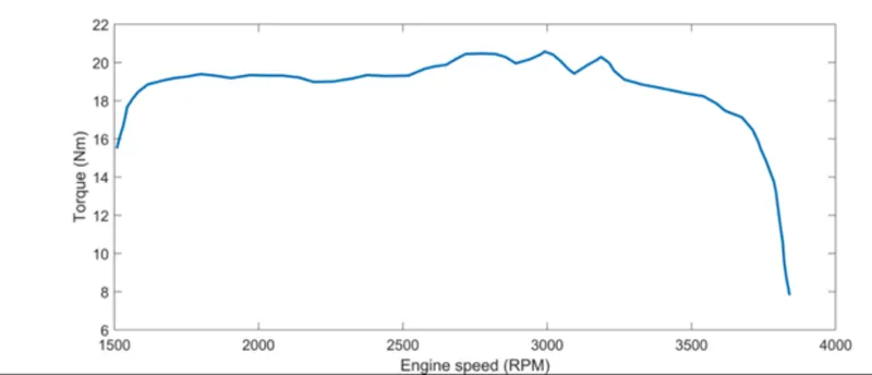
So, BAJA ATV model without Dashboard is simulated and the input,output and Speed vs torque plots are shown in the report.
Case2: BAJA ATV model with Dashboard.
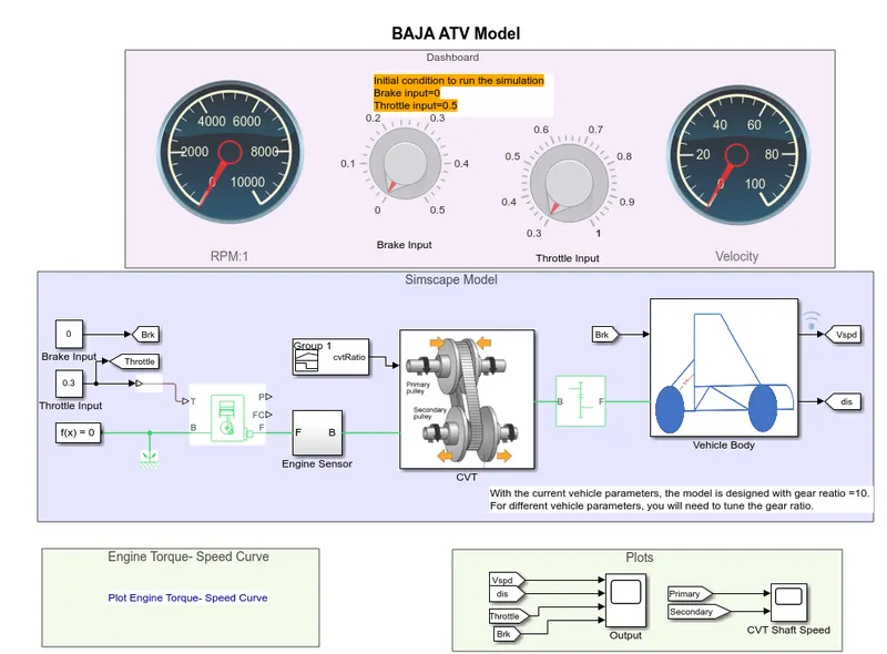
Simulink block and parameters will be same as BAJA ATV Model Without dashboard,but input values for brake, throttle and cvt ratio may varies according to model given in the example.
Dash board used to control or vary the input signals using a knob as shown in the model. And the Custom gauge is used to indicate the variation of speed and velocity when the brake and throttle input is changing by using knobs.
Simulink Model:
Cvt Input gear ratio:
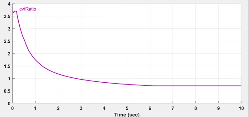
Plot shows the input gear ratio to CVT, which is created using signal builder.
Output Scope:
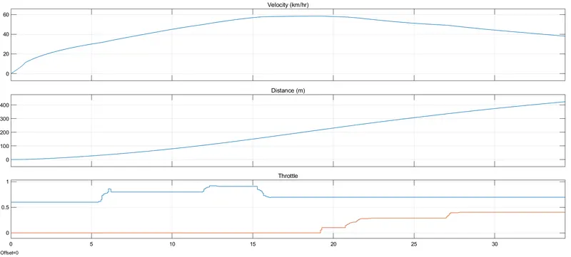
1. Plot shows the vehicle velocity, distance travelled , throttle input and brake input to the generic engine block.
2. From the graph we can observe that, the initial values of throlled input and brake input is 0.55 and 0 respectively. when we start simulation velocity of the vehicle is increasing trend. after 5 sec if we increase the throttle input, we can observe the change in velocity is in increasing trend nad when we reduce the throttle input the velocity starts reducing slowly. In the same way if we increase the brake signal using knob during simulation time, we can observe the after 18 sec, when brake signal is applied the velocity starts in decreasing trend.
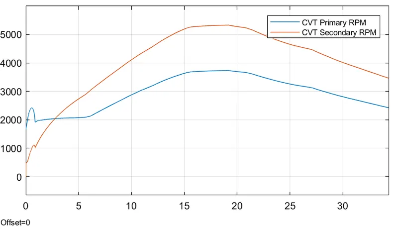
3. CVT primary shaft rpm and secondary shaft rpm is shown below. the variation of secondary and primary rpm can be observed when the throttle and brake inputs applied.
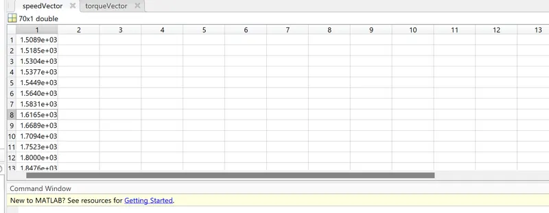
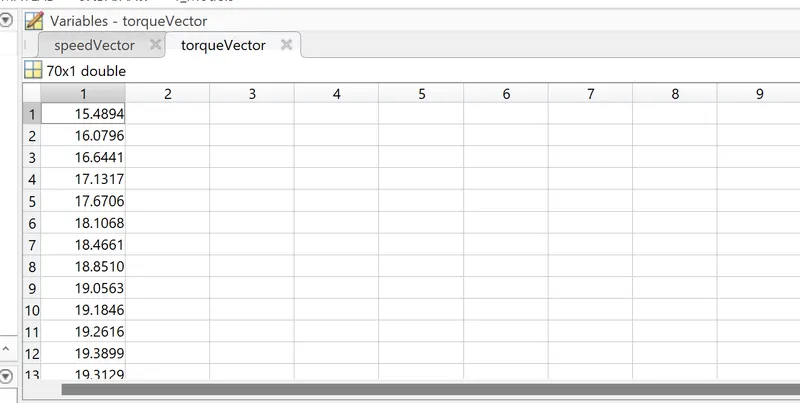
Torque vector and speed vectors are saved in work shop and the data is shown below,
Speed vector data:
Torque vector:
Using the speed and torque vectors data,plot of Speed vs torque will be similar to the graph plotted below
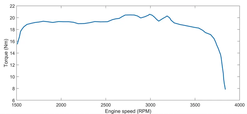
So, BAJA ATV model using Dashboard is simulated and th input,output and Speed vs torque plots are shown in the report.
Case3:BAJA ATV Model uses Lookup table without Dashboard.
Block for the model created is same as case2 study,but the one change is lookup table used for describing the cvt gear ratio to the input of CVT instead of Signal builder.
Lookup table: A look up table is an array of data that maps input values to output values, thereby approximating a mathematical function. For a given set of values a lookup operation retrieves the corresponding output values from the table. If the lookup table doesnot explicitly define the input values Simulink can estimate an output value using interpolation, extrapolation or rounding.Here,
An Interpolation is a process for estimationg values that lie between known data points.
An exterpolation is a process for estimating values that lie beyond the range of known data points.
A rounding is aprocess for approximating a value by altering its digits according to the known values.
Lookup table outuput or cvt ratio plot is shown below,
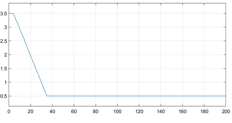
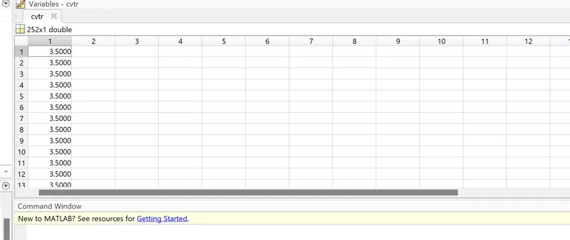
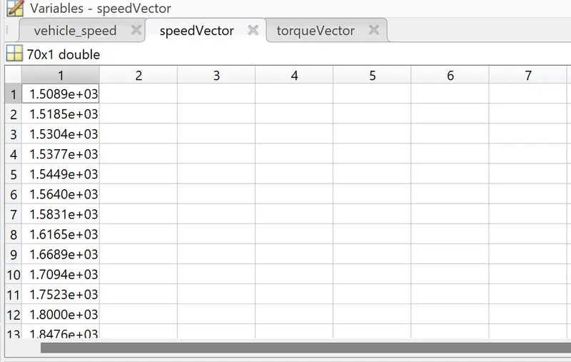
CVT values are saved in the lookup table is shown below and these are saved into workspace.
CVT Block using Lookup Table:
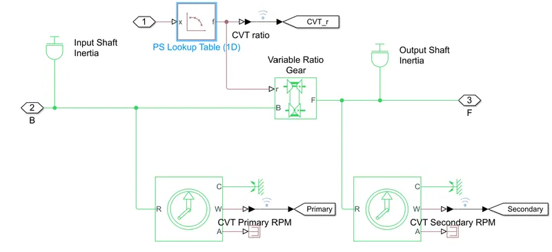
CVT ratio is obtained from the lookup table. Input shaft represents the primary pulley and output shaft represents the secondary pulley and mechanical rotational sensors is connected to input and output shafts.Variable ratio gear represents variable gear ratio gearbox such as implemented by belt CVT , electrical or hydraulic transmissions.The physical input R defines the ratio of input to output angular shaft velocities. Connections B and F are mechanical conversing ports.
Scope: Plot shows the graph of parameters velocity,throttle input and brake input.
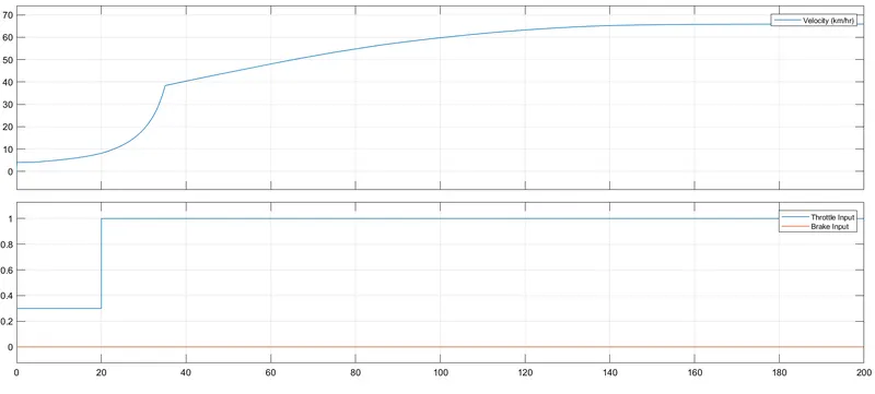
Plot Shows the wheel throttle is at 0.3 for 20 sec speed of vehicle is increasing correspondingly and at full throttle that is at 1 the vehicle speed is jumped nearly to 40 kmph and then increases proportionally and the result remains same as the input parameter remains same.
CVT output Scope:
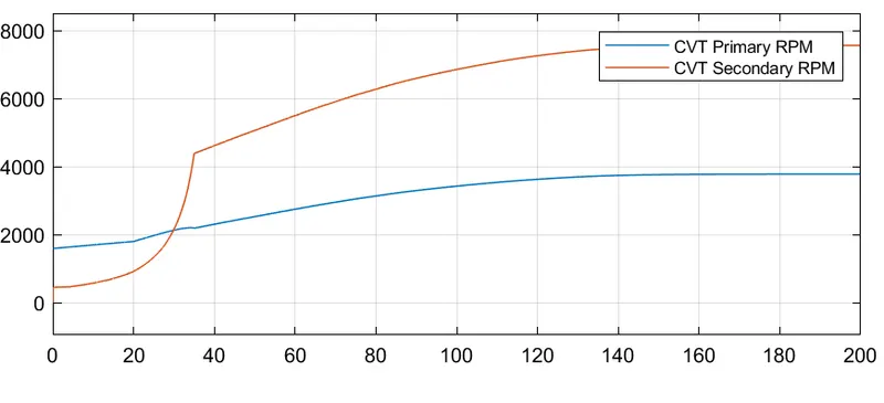
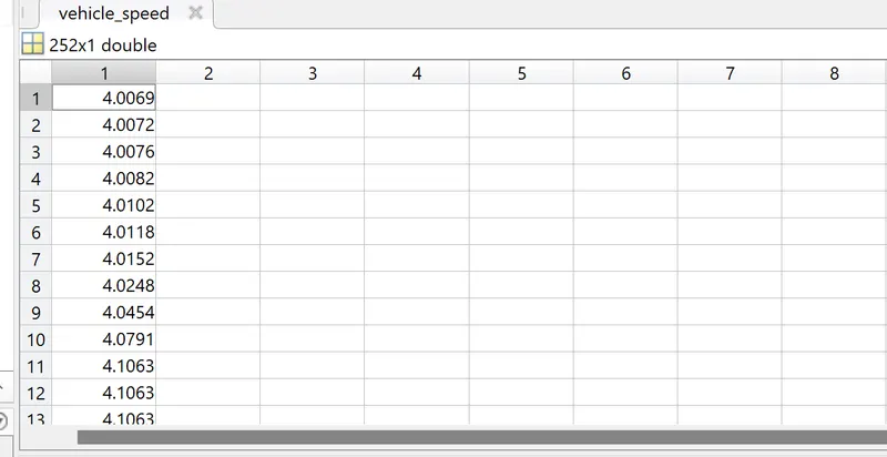
From the plot it is observed that the secondary of CVT speed and the velocity plot will be same as above plot. and the velocity of vehicle speed data stored in the workspace is shown below
Speed and torque vectors saved in the workspace is shown below,
torque vector data:
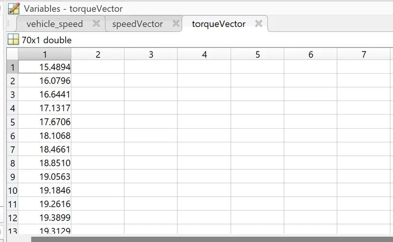
Speed vector data:
Plot of torque vector Vs speed vectors is shown below using the saved data from the workspace,
So, BAJA ATV model using Lookup table without Dashboard is simulated and th input,output and Speed vs torque plots are shown in the report.
Case:4 BAJA ATV model using Lookup table with Dashboard.
The study is based on the BAJA ATV model using lookup table with dashboard is shown in the below figure. In this model also blocks used are same as case3, but the inputs of brake and throttle is provided using knobs and speed and velocity is shown using custom gauge. This study is mainly to undestand the variation in speed nad velocity by varying the brake and throttle input during simulation time.
CVT Ratio :
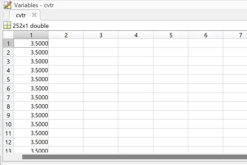
CVT ratio data created in workspace is shown below,
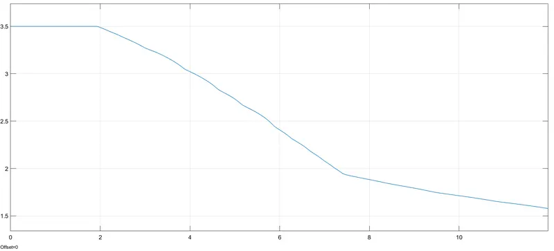
CVT ratio input using lookup table is shown below,
Scope output for velocity ,brake and throttle inputs:
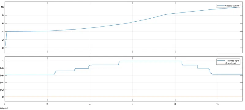
We can clearly obsorve as the throttle input increasing the velocity of vehicle also increased proportionally and when it goes to 1 the velocity is gradually going to be stable and if we reduce the throttle input, the velocity reduces as hown in the graph. As we didnot vary the brake input using the knob the graph shows zero.
Engine Speed:
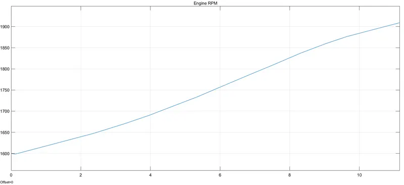
Engine speed is connected to the CVT input port i.e., Base so the CVT primary RPM and the Engine RPM will be almost similar as shown in the graph.
CVT Shaft Speed:
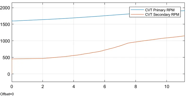
From the above graph it is cleary obsorved the velocity of vehicle and the secondary rpm of CVT is same, as the output of CVT is connected to the vehicle.
Vehicle Speed:
Vehicle speed recorded in the workspace is shown below,
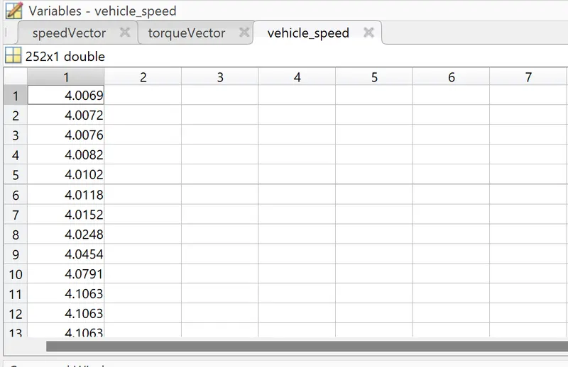
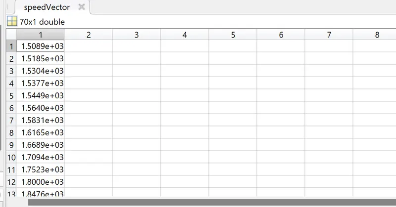
Speed and torque vectors saved in the workspace is shown below,
Speed Vector data :
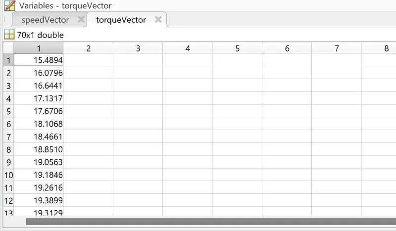
Torque vector data:
Plot of torque vector Vs speed vectors is shown below using the saved data from the workspace,
So, BAJA ATV model using Lookup table with Dashboard is simulated and the input-output plots are shown in the report.
Conclusion:
Hence the BAJA ATV terrain vehicle model was simulated successfully and from the above results we can conclude that,
- Velocity, CVT shaft Speed and Engine speed are directly proportional to the throttle input and inversely proportional to the brake input.
-If the brake input is at high, at particular point the vehicle speed may become zero.
-As the CVT secondary shaft is connected to the Vehicle input, the speed of CVT Shaft and vehicle will be almost similar.