Project
OBJECTIVE:
The main objective of this project is to carry out a system-level simulation of an all-terrain vehicle. The model must be studied and explained for each step that is carried out during the simulation.
MODEL SIMULATION AND EXPLANATION:
ALL-TERRAIN VEHICLE:
An all-terrain vehicle is defined as a motorized off-highway vehicle designed to travel on four low-pressure or non-pneumatic tires, having a seat designed to be straddled by the operator and handlebars for steering control.
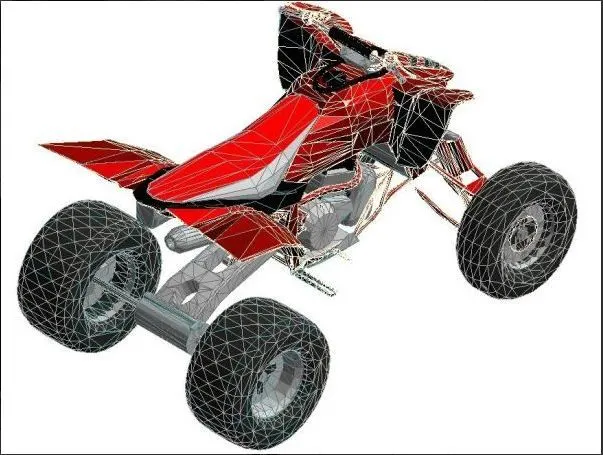
Fig.1: Model of ATV(All-terrain vehicle)[1]
CONTINUOUSLY VARIABLE TRANSMISSION:
A continuously variable transmission (CVT) is an automatic transmission that can change seamlessly through a continuous range of gear ratios. This contrasts with other transmissions that provide a limited number of gear ratios in fixed steps. The flexibility of a CVT with suitable control may allow the engine to operate at a constant RPM while the vehicle moves at varying speeds.
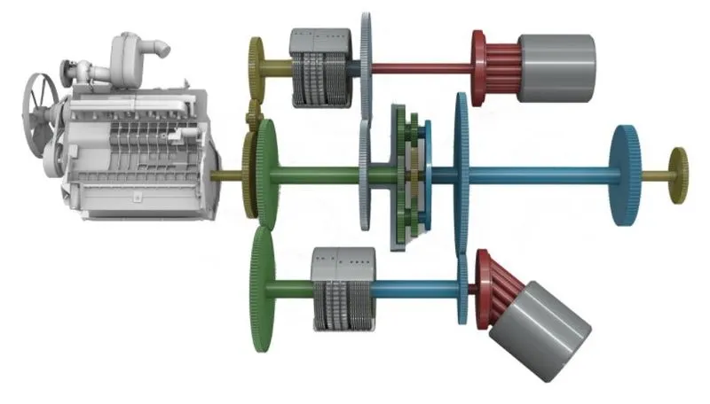
Fig.2: Continuous Variable transmission[2]
BAJA ATV Model[3]
The list of the entire model structure is mentioned below
MODELS:
- cvtModel.slx - Contains Simscape model of BAJA ATV with Continuous Variable Transmission.
- cvtModel_dashboard.slx - The model is similar to, "cvtModel" with addition of dashboards.
MODELS_LOOKUPTABLE:
- cvtModel_cvtratio_rpm.slx - Contains model based on cvt ratio and engine rpm lookup table.
- cvtModel_mapped.slx - Contains Simscape model of BAJA ATV with Continuous Variable Transmission where the CVT ratio varies based on 1D lookup table.
- cvtModel_dashboard_mapped.slx - The model is similar to, "cvtModel_mapped" with the addition of dashboards.
- cvtModel_data.slx - The model is used to log the CVT ratio and vehicle speed for the look table visualization
- lookuptable_visualization.m - Script to load and run the model, "cvtModel_data".
The area of the Simulink model is split into
- Simscape model – Entire model of the ATV
- Plots – Outputs connected to the scope
- Engine Torque Vs Speed Curve – Annotation converted to Plot using Clickfn from the input defined in callback
cvtModel.slx:
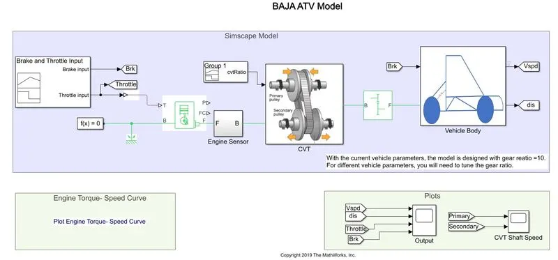
Fig.3: Simulink model- cvtModel
Simscape Model:
Inputs:
Signal Builder:
This is the commonly used input block for custom-made inputs and the number of inputs can also be controlled by adding and deleting signals. Here two signals, Brake input, and Throttle input is given as input.
The inputs like m1, m2, mr1, mr2, speedVector, torqueVector are pre-defined in the callback function.
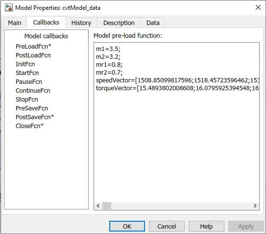
Fig.4: Pre-load function of the model
Brake output is initially set to zero throughout the simulation. So, when the value of the brake is changed there can be a change in the rpm of the engine crankshaft can be identified.
Throttle (value is always between 0 and 1) is given to the Engine to get the rotation of the Engine crankshaft which is then connected Engine sensor to calculate the rpm of the crankshaft.
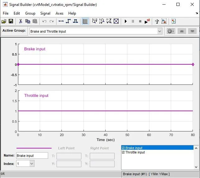
Fig.5: Signal builder input for throttle and brake
Generic Engine:
This Mechanical Simscape block acts as a simple spark engine where throttle and the engine block are given as input and the engine block is connected to the Mechanical Rotational reference. Using this block, the parameters like Engine power and fuel consumption rate can also be visualized as output. The engine crankshaft is the major output as the rotation of the crankshaft increases as the throttle value increases.
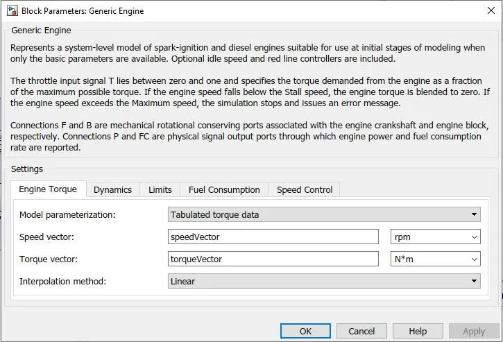
Fig.6: Generic engine block main Parameters
Signal Builder:
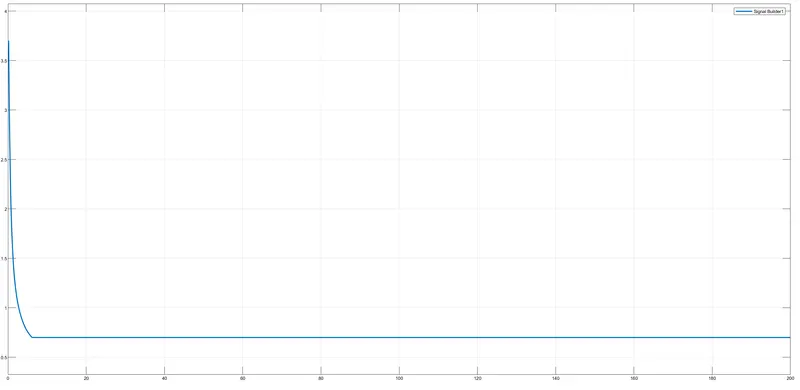
CVT Ratio – It is the ratio of input to the output angular velocities. The .MAT (CvtRatio.mat) file is imported to the signal builder from the import from file option and the data is selected.
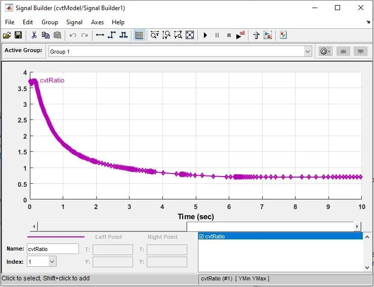
Fig.7: CVT ratio - Signal Builder input model 1
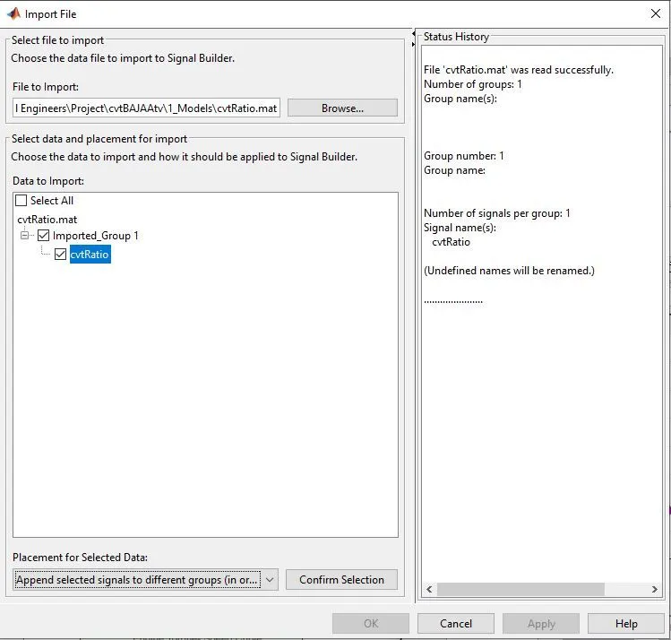
Fig.8: Import .MAT file in Signal builder
Engine Sensor Subsystem:
A separate subsystem is created to measure the rpm (revolutions per minute) of the engine crankshaft using an ideal rotational motion sensor.
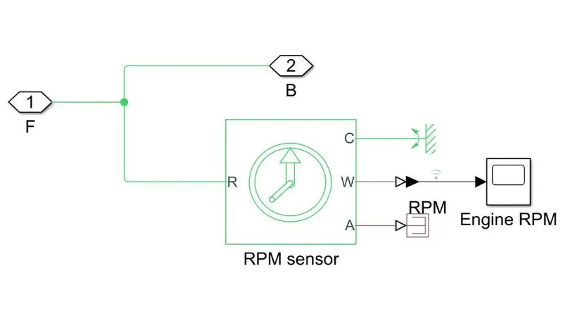
Fig.9: Engine Sensor Subsystem
CVT Subsystem:
CVT subsystem increases the speed of the engine using the variable gear ratio. Inertias are very important to this model because they can control the change in the speed of the engine crankshaft.
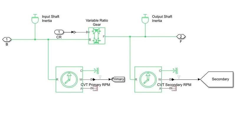
Fig.10: CVT subsystem
Inertia:
Inertia refers to resistance to change — in particular, resistance to changes in motion.
Variable Gear Ratio:
Variable-ratio gear pair refers to the one which could produce a variable rotational motion between two connected drive shafts in a transmission. It is mainly applicable to meet the demand for special mechanical transmission, such as continuously variable transmissions (CVTs) in vehicles.
Simple Gear:
This is a simple two gear block where the input block is directly connected to the secondary output of the CVT subsystem. The ratio given here is 10. So, the follower gear rotates according to the base gear.
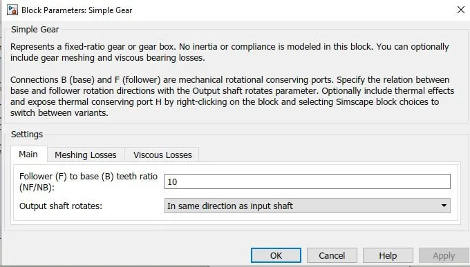
Fig.11: Parameters - Simple Gear
Vehicle body Subsystem:
The inputs of this subsystem are the Brake value from the initial Signal builder and follower gear rotation.
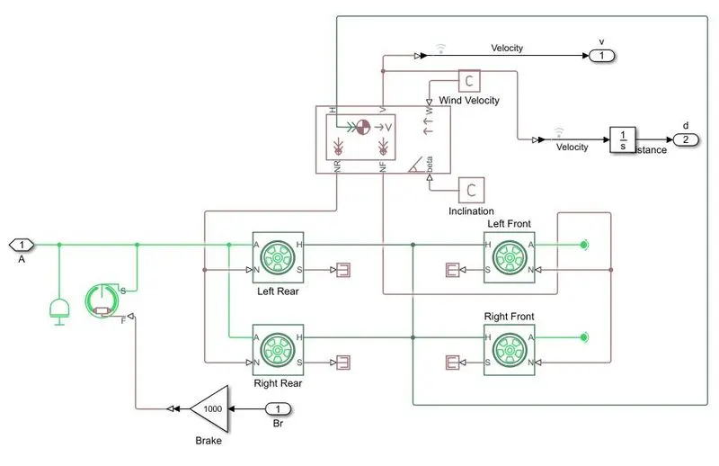
Fig.12: Vehicle Body Subsystem
As the model shows this is a Rear Transmission vehicle, where the acceleration input is given from the follower gear which controls both the rear wheels.
A double shoe brake is used as the braking system for the vehicle. A gain of 1000 is given because the values are in the range of 0 to 1.
An inertia block is used again here to resist the rotation of the follower gear in the simple gear.
Vehicle body block is used to connect the normal forces of the rear and front wheels. Similarly, all the horizontal ports of all the wheels and the vehicle body are connected for the horizontal motion of the vehicle. Also, from this block velocity of the vehicle can be found. Input for wind velocity and the inclination angle of the road also can be given to simulate at different conditions.
Usually, an integrator block is used to change the velocity value to distance and both the values of the vehicle are visualized in scope.
Plots:
Using from the block all the required outputs like Speed of the vehicle (Vspd), distance covered(dis), Throttle input, Brake input, Primary rotation of the engine, and secondary rotation of the engine (after converting it using variable gear ratio).
cvtModel_dashboard.slx:
With Dashboard
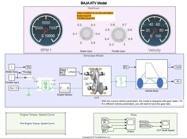
Fig.13: Simulink model- cvtModel with dashboard
The main difference between the model with dashboard and without dashboard is the simulation time and the inputs like throttle and brake. Where cvtModel.slx is run for 200 seconds and cvtModel_dashboard.slx is run for infinite time so that the parameters can be changed during the run time and spontaneous change in the results can be visualized.
This is the overall execution strategy of the model and only the inputs to the CVT subsystem are changed for other models and are explained below in a table.
cvtModel_cvtratio_rpm.slx:
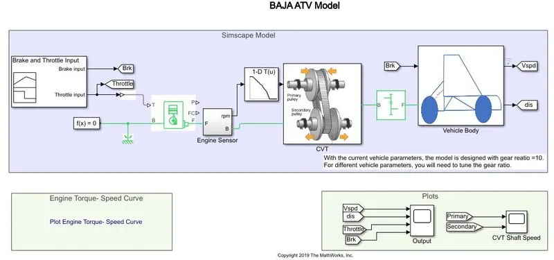
Fig.14: Simulink model- cvtModel_cvtratio_rpm
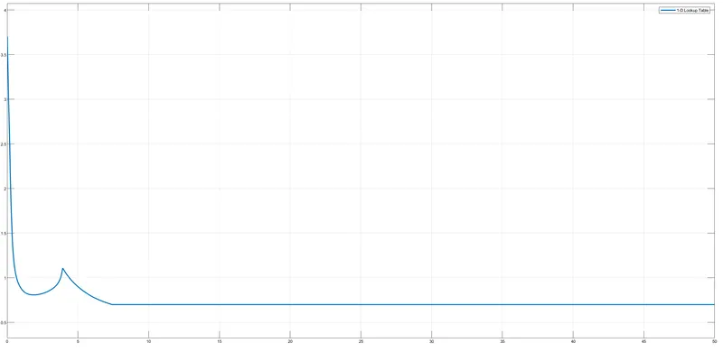
The overall model is shown above and the lookup input is given to the CVT subsystem and rpm data from the Engine block subsystem is given as input to the lookup table from the Simulink system and the breakpoints are given from the .MAT file specified.
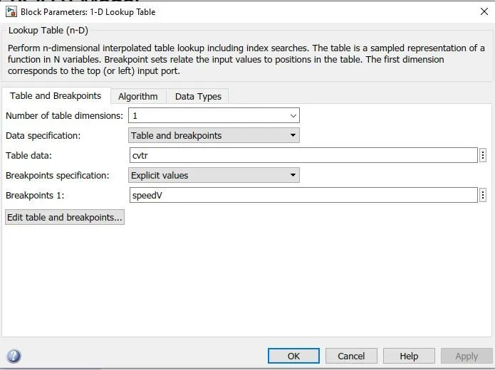
Fig.15: 1D Lookup table- Simulink
cvtModel_data.slx:
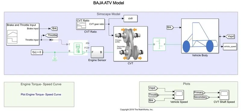
Fig.16: Simulink model - cvtModel_data
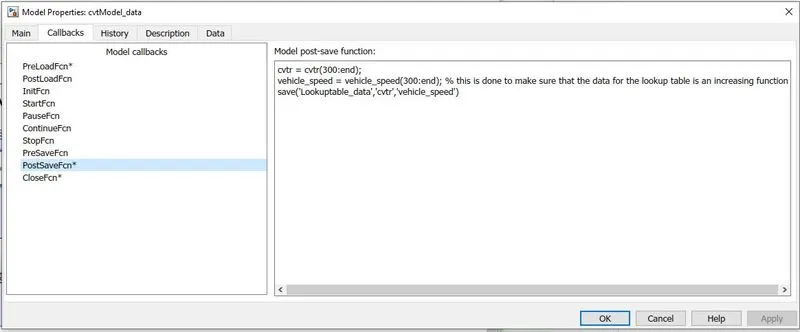
Fig.17: Post save function
cvtModel_mapped.slx:
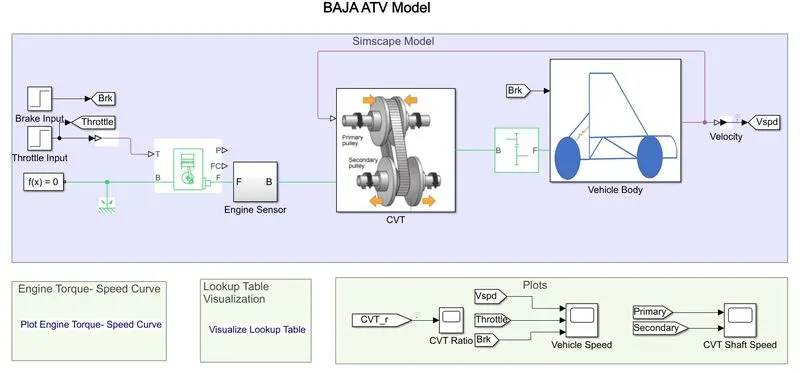
Fig.18: Simulink model - cvtModel_mapped
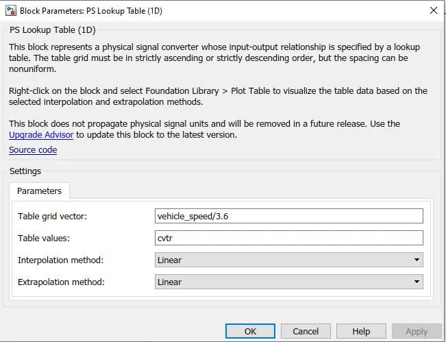
Fig.19: 1D Lookup table PS(Physical Systems)
cvtModel_dashboard_mapped.slx:
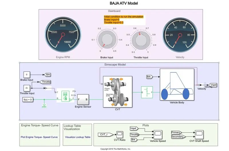
Fig.20: Simulink Model - cvtModel_dashboard_mapped
|
Model |
Throttle Input |
Brake Input |
CVT ratio |
CVT Ratio graph |
Rpm Input |
Simulation Time |
|
cvtModel.slx |
Signal Builder (manually defined) |
Signal Builder (manually defined) |
Signal Builder (Imported from cvtRatio.MAT file) |
Fig.21: CVT ratio from Signal builder(model 1) |
No |
200 secs |
|
cvtModel_dashboard.slx |
Constant block connected to knob in dashboard |
Constant block connected to knob in dashboard |
Signal Builder (Imported from cvtRatio.MAT file) |
Fig.22: CVT ratio from Signal builder(model 2) |
No |
inf |
|
cvtModel_cvtratio_rpm.slx |
Signal Builder (manually defined) |
Signal Builder (manually defined) |
From 1D lookup table (Simulink) for the data from Lt_cvratio_rpm.MAT |
Fig.23: CVT ratio from Lookuptable (Simulink) |
Yes, from the Engine Sensor subsystem |
50 secs |
|
cvtModel_data.slx |
Signal Builder (manually defined) |
Signal Builder (manually defined) |
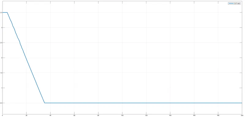
Signal Builder(manually controlled). A postsavefcn is used to save cvrt after 300 step-time and visualized in workspace |
Fig.24: CVT ratio from Signal builder(model 4) |
No |
200 secs |
|
cvtModel_mapped.slx |
Step Input block |
Step Input block |
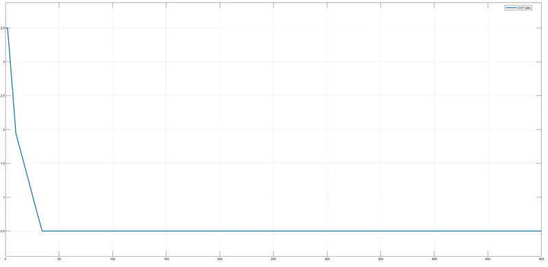
From 1D lookup table (Physical Systems) for the data from Lookuptable_data |
Fig.25: CVT ratio from Signal builder(model 5) |
No |
200 secs |
|
cvtModel_Dashboard_mapped.slx |
Constant block connected to knob in dashboard |
Constant block connected to knob in dashboard |
From 1D lookup table (Physical Systems) for the data from Lookuptable_data |
Fig.26: CVT ratio from Lookuptable (PS) |
No |
inf |
OUTPUTS:
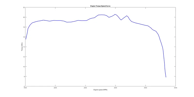
Fig.27: Engine Speed Vs Torque
Velocity, Inputs (Throttle and Brake):
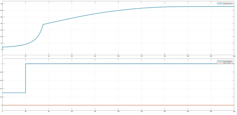
Fig.28: [Velocity, Throttle, Brake] Vs Time
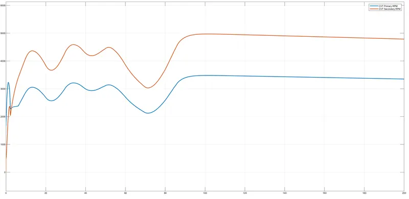
Fig.28: [Primary shaft speed, Secondary shaft speed] Vs Time
CONCLUSION:
Thus the system-level simulation of every model(ATV) was executed and the difference between each model was analyzed.
REFERENCES:
[1] https://www.cadblocksfree.com/de/raptor-atv-revit-family.html
[3] https://ch.mathworks.com/matlabcentral/fileexchange/70576-baja-all-terrain-vehicle-atv-model