Week 4.1 - Genetic Algorithm
Objective:
The main objective of this challenge is to implement the genetic algorithm optimization for the stalagmites in MATLAB and try for different optimization options to get better results.
Genetic Algorithm(GA)
GA is a search-based optimization technique based on the principles of Genetics and Natural selection. It is frequently used in the determination of optimal solutions for difficult problems that may require a long time to solve (E.g., Growth of a Stalagmite) or in situations where a solution is impossible.
Optimization usually refers to making something better. It also refers to finding the values of inputs so that the best values for the outputs are achieved. Search space is the set of all possible solutions or values which the inputs can take. In this search space lies a single point or set of points that gives the optimal solution. This is the aim of optimization in GA.
The step by step procedure for Genetic algorithm optimization is explained below:
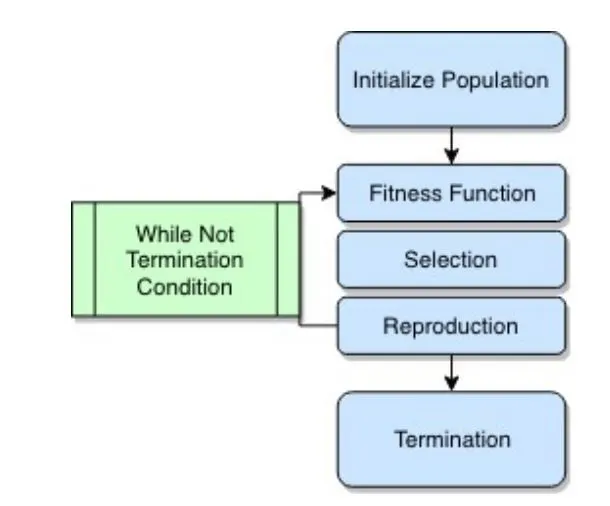
Fig.1: Flow chart of Genetic Algorithm[1]
Step 1: Initialize Population
This step begins with guessing the initial set of values that may or may not contain the optimal values in the search space area.
Step 2: Fitness function
Fitness function is the heart of the genetic algorithm. In this challenge, we use the equations for the stalagmite. This function takes an individual point and determines how well it fulfills whatever criteria the algorithm is optimizing for.
Step 3: Selection function
This process retains the best performing values or bit strings from one generation to the next. The Selection function takes the population and the results of the fitness function to determine what to reproduce. If a threshold value is set for reproduction, then the selection function filters the population by the threshold value.
Step 4: Reproduction Function
This function determines how to expand the population based on the existing conditions and how the population changes over time. Modifying the behavior and parameters of the reproduction function is one of the most complex parts of generating a genetic algorithm. There are two methods in reproduction function:
Mutation function: This is a simple method where each new member is based on a single individual. When doubling the population, each individual creates a new individual with the same characteristics modified by a random factor.
Crossover function: This is a more complex method of reproduction, where each individual is based on some combination of existing individuals.
The reproduction function returns the new population, which may be the same size or a different size than the original population.
Step 5: Termination Function
After the desired number of iterations have occurred, this function takes the ending population and returns the best members by the fitness score.
Stalagmites-General Information:[2]
Stalagmites are a wonderful example of nature’s sculpturing. They are formed because of rainwater that seeps through the caves over a period. Stalagmites grow upwards from the cave floor and look like cones. They usually grow at a very slow rate, approximately around one inch per year. The rate of growth depends on two factors,
- Temperature outside the cave
- Amount of Rainfall in the region
The shape of these minerals is determined by the way the acidic water enters the cave and the colour is determined by the mineral content. Pure calcite is white and often colourless. Iron and other minerals as well as acids from ground vegetation, combine with calcite crystals to form different hues of red, orange, and black colours.
Stalagmites are abundantly found in caves of California and France. In India, they are found in Araku valley caves in Andhra Pradesh and old caves in Meghalaya.
Some formulas used in fitness function using stalagmites for genetic algorithm are
`f_(1,x) = [sin(5.1 * pi * x + 0.5)]^6`
`f_(1,y) = [sin(5.1 * pi * y + 0.5)]^6`
`f_(2,x) = exp(-4 * ln(2)* ((x-0.0667)^2/0.64))`
`f_(2,y) = exp(-4 * ln(2)* ((y-0.0667)^2/0.64))`
The final function is , `f(x,y) = f_(1,x) * f_(1,y) * f_(2,x) * f_(2,y)`
Genetic Algorithm in MATLAB:
ga syntax in MATLAB:
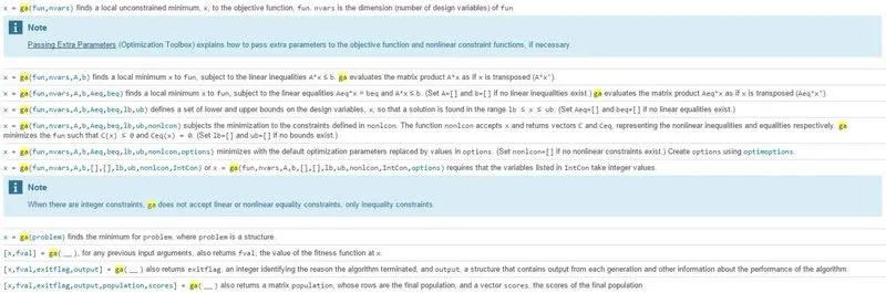
Code for Genetic Algorithm:
clear all;
clc;

%% Defining Inputs - Search Space
X = linspace(0,0.6,150);
Y = linspace(0,0.6,150);

%% Creating 2D Mesh
[XX, YY] = meshgrid(X, Y);

%% Evaluating Stalgamite function (Fitness Function)
for i = 1:length(XX)
    for j = 1:length(YY)
        ip_Vec(1) = XX(i,j); % inputs from x
        ip_Vec(2) = YY(i,j); % inputs from y
        f(i,j) = stalagmite(ip_Vec); % Execution of stalagmite.m
    end
end

figure(1)
surfc(XX,YY,f) % Contour 3D shaded plot
shading interp; % Eliminates gridlines and provides smoother shading to the plot for better view
colormap(parula); % color used in plot is PARULA(a colour combination from a bird)
colorbar('Axislocation','out'); % Legend bar with axis pointing outwards
[Max, fval] = ga(@stalagmite,2) % Execution of ga syntax
% Without a loop only two values can be extraced from the ga syntax
B_X = Max(1)
B_Y = Max(2)
xlabel('X axis search space')
ylabel('Y axis search space')
zlabel('Maxima of the function')


%% Define the number of iterations for GA
% Dialog box Creation to specify the iteration of GA
prompt = {'Number of iteration Desired:'}; % Inputs specified for the split
dlgtitle = 'Genetic Algorithm Iteration'; % Name of the dialog box
dims = [1 55]; % dimension of the dialog box
definput = {'50'}; % default numbers in the input area
answer = inputdlg(prompt,dlgtitle,dims,definput); % Creating the dialog box and given i/p are saved as cell array
n = str2double(answer); % converting it to number(iteration)


%% STUDY 1 : Undefined Boundary Conditions
% No boundary conditions are dedfined and loop to execute the number of
% iterations specified
Start_Study1 = tic; % start of stop clock for study 1
for p = 1:n
    [Max, fvals1(p)] = ga(@stalagmite,2); % fvals is the Maxima points data for each iteration
    B_Xs1(p) = Max(1); % function values of X
    B_Ys1(p) = Max(2); % function values of X
end
Study_1_Time = toc(Start_Study1); % stop of stop clock for study 1
fprintf('Time of Execution for study 1\n %d Min and %f Secs\n', floor(Study_1_Time/60), rem(Study_1_Time,60))

figure('Name','Study Case 1: Undefined Boundary Conditions')
subplot(2,1,1)
surfc(XX,YY,f)
shading interp;
colormap(parula);
colorbar('Axislocation','out');
hold on
% 3D plot to show the maxima points in the study
plot3(B_Xs1,B_Ys1,fvals1,'--r','Marker','o','MarkerSize',6,'MarkerFaceColor','k')
xlabel('X axis search space')
ylabel('Y axis search space')
zlabel('Maxima of the function')
title('Study Case 1: Undefined Boundary Conditions')
hold off
subplot(2,1,2)
% Plot to show maxima point at each iteration
plot(fvals1)
xlabel('Iterations')
ylabel('Maxima Function:Study 1')


%% STUDY 2: Defined Boundary Conditions
Start_Study2 = tic;
for p = 1:n
    [Max, fvals2(p)] = ga(@stalagmite,2,[],[],[],[],[0;0],[0.6;0.6]);
    B_Xs2(p) = Max(1);
    B_Ys2(p) = Max(2);
end
Study_2_Time = toc(Start_Study2);
fprintf('Time of Execution for study_2 is\n %d Min and %f Secs\n', floor(Study_2_Time/60), rem(Study_2_Time,60))

figure('Name','Study Case 2: Defined Boundary Conditions')
subplot(2,1,1)
surfc(XX,YY,f)
shading interp;
colormap(parula);
colorbar('Axislocation','out');
hold on
plot3(B_Xs2,B_Ys2,fvals2,'--r','Marker','o','MarkerSize',6,'MarkerFaceColor','k')
xlabel('X axis search space')
ylabel('Y axis search space')
zlabel('Maxima of the function')
title('Study Case 2: Defined Boundary Conditions')
hold off
subplot(2,1,2)
plot(fvals2)
xlabel('Iterations')
ylabel('Maxima Function: study 2')


%% STUDY 3: Defined Boundary Conditions and other important Parameters
options = optimoptions('ga','populationsize',300,'ConstraintTolerance',1e-6,'PlotFcn', @gaplotbestf);
% PlotFcn command is used to optimize the plot to find the best value for each iteration(It undergoes the iteration for a certain number of times where the best value is achieved each time)
% ConstrainTolerence is the tolerance value of the maxima point in the range of 10e-6
% population size is the total of the population available for optimization

Start_Study3 = tic;
for p = 1:n
    [Max, fvals3(p), e_flag, optut, popu, score] = ga(@stalagmite,2,[],[],[],[],[0;0],[0.6;0.6],[],[],options);
    B_Xs3(p) = Max(1);
    B_Ys3(p) = Max(2);
end
Study_3_Time = toc(Start_Study3);
fprintf('Time of Execution for study_3 is\n %d Min and %f Secs\n', floor(Study_3_Time/60), rem(Study_3_Time,60))

figure('Name','Study Case 3: Defined Boundary Conditions and other Parameters')
subplot(2,1,1)
surfc(XX,YY,f)
shading interp;
colormap(parula);
colorbar('Axislocation','out');
hold on
plot3(B_Xs3,B_Ys3,fvals3,'--r','Marker','o','MarkerSize',6,'MarkerFaceColor','k')
xlabel('X axis search space')
ylabel('Y axis search space')
zlabel('Maxima of the function')
title('Study Case 3: Defined Boundary Conditions and other Parameters')
hold off
subplot(2,1,2)
plot(fvals3)
xlabel('Iterations')
ylabel('Maxima Function: Study 3')
Study 1: Undefined boundary Conditions
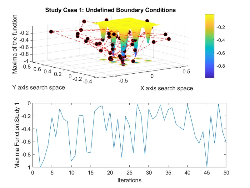
Fig.3: Output Study 1(Undefined boundary conditions)
Study 2: Boundary Conditions defined
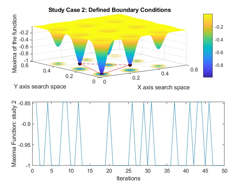
Fig.4: Output Study 1(Defined boundary conditions)
Study 3: Boundary condition and Population defined
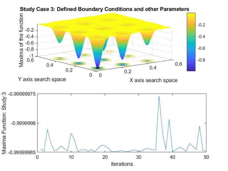
Fig.5: Output Study 1(Defined boundary conditions and population)
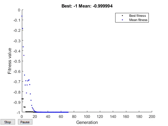
Fig.6: A graph using PlotFcn for the last iteration
The graph above shows the best value computing the running mean and plotting Generation Vs Fitness value for getting a better value for the maxima point. So the execution time of the last study may take a little bit longer but with accurate results.
Conclusion:
The following were achieved in this challenge
- A genetic algorithm(optimization) was studied and implemented in MATLAB.
- Maxima function was found using the ga syntax.
- Three study cases were explained with different conditions and the results were analyzed and optimized.
References:
[1] https://blog.floydhub.com/introduction-to-genetic-algorithms/