Challenge

Project 2 - Rankine cycle Simulator

RRamkumar Ganesan Rajalekshmi7 Sept 2021

OBJECTIVE:

The main objective is to write a MATLAB code to simulate the working of the Rankine Cycle.

THEORY AND IMPLEMENTATION:

Rankine cycle is a vapor power cycle.

A power cycle is a cycle that uses heat to generate work. As the Rankine cycle is based on vapor, it uses steam to rotate the blades of the turbine.

It utilizes the heat energy contained in coal, oil, or natural gas and then converts it into mechanical energy and eventually into electrical energy.

Rankine cycle is derived from the Carnot cycle which closely describes the process of Steam Turbine systems. Carnot cycle is the most efficient thermodynamic cycle which explains Power is dependent on the hot sources and cold sources (our surroundings). The higher the difference, the more mechanical power can be efficiently extracted out of heat energy.

Types of Rankine Cycle:

Reheat: introduce exhausted steam back into the boiler to reheat it
Regenerative: bled a part of steam into heat exchangers to preheat the feed water before entering the boiler
Organic Rankine: Uses organic high molecular mass fluid with a boiling point occurring at a lower temperature than the water-steam phase change.
Supercritical: Water is the working fluid and operated above its critical pressure

IDEAL RANKINE CYCLE:

This is a reversible cycle. Constant pressure or isobaric process and constant entropy or isentropic process are used by equipment involved in this cycle.

NEGLECTED:

Frictional pressure drops and
undesired heat transfer with surroundings

Process 1-2: Isentropic Expansion The Vapor is expanded in the turbine, thus producing work that may be converted to electricity.

Process 2-3: Isobaric Heat Rejection The vapor-liquid mixture leaving the turbine is condensed at low pressure. In these condensers, the pressure of the vapor is below the atmospheric pressure, approaching the saturation pressure of the operating fluid at the cooling water temperature.

Process 3-4: Isentropic Compression The Pressure of the condensate is raised in the feed pump. Because of the low specific volume of liquids, the pump work is relatively small and often neglected in thermodynamic calculations.

Process 4-1: Isobaric Heat Transfer High-Pressure liquid enters the boiler from the feed pump and is heated to the saturation temperature. Further addition of energy causes evaporation of the liquid until it is fully converted to saturated steam.

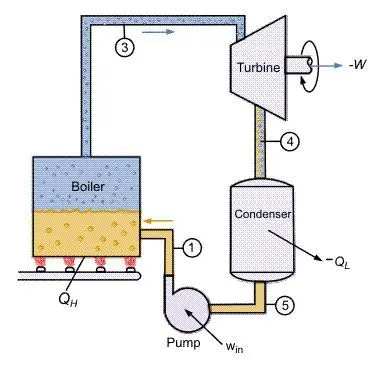
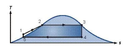
Fig.1: Rankine Cycle Fig.2: T-S diagram of Rankine Cycle

Thermal Efficiency:

It is defined as the ratio of Net-work done to the Heat addition.

Back Work Ratio:

The ratio of the compressor work to the turbine work.

The MATLAB code to run the details regarding the Rankine cycle is:

%% Creating list of Rankine cycles
list = {'Basic Rankine Cycle','Reheat','Regenerative',...
    'Organic','Supercritical'};
[indx,tf] = listdlg('PromptString',{'Select a cycle to know about it!!.'},...
    'SelectionMode','single','ListString',list);

%% Condition to view each cycle
% Simple Rankine
if indx == 1
    figure('Name','Simple Rankine Cycle')
    sgtitle('Information about Simple Rankine Cycle')
    fi = imread('Rank_ideal.JPG');
    subplot(2,1,1)
    imshow(fi);
    subplot(2,1,2)
    ylim([0 100])
    hold on
    text(0,100,['Rankine cycle is derived from Carnot cycle which closely'])
    text(0,90,['describes the process of Steam Turbine systems. Carnot'])
    text(0,80,['cycle is the most efficient thermodynamic cycle which'])
    text(0,70,['explains Power is dependent on hot source cold source'])
    text(0,60,['(our surrounding). The higher the difference, the more'])
    text(0,50,['mechanical power can be efficiently extracted out of heat energy.']); axis off
    hold off
    pause(5)

    % Reheat
elseif indx == 2
    figure('Name','Reheat Rankine Cycle')
    sgtitle('Information about Reheat Rankine Cycle')
    fi = imread('Reheat.JPG');
    subplot(2,1,1)
    imshow(fi);
    subplot(2,1,2)
    ylim([0 100])
    hold on
    text(0,100,['This Rankine cycle introduce the exhausted steasm back '])
    text(0,90,['into the boiler to reheat it. At the next stage, the reheated'])
    text(0,80,['stem will go past another turbine to produce more work.'])
    text(0,70,['Steam from the boiler will expand in a high-pressure turbine.'])
    text(0,60,['Since the turbine pressure is high steam that comes out of the turbine'])
    text(0,50,['will have higher pressure in contrast to the normal Rankine cycle.']); axis off
    hold off
    pause(5)
  
    % Regenerative
elseif indx == 3
    figure('Name','Regenerative Rankine Cycle')
    sgtitle('Information about Regenerative Rankine Cycle')
    fi = imread('Regenerative.JPG');
    subplot(2,1,1)
    imshow(fi);
    subplot(2,1,2)
    ylim([0 100])
    hold on
    text(0,100,['This Rankine cycle bled a part of steam into heat exchangers'])
    text(0,90,['to preheat the feedwater before entering the boiler.Feeding the '])
    text(0,80,['water at a relatively high temperature can increase the overall '])
    text(0,70,['efficiency of the cycle. Condensed water along with partially expanded '])
    text(0,60,['steam will mix in a heat exchanger to produce water at a high temperature.'])
    text(0,50,['The mixture will be pumped into the boiler to repeat the cycle.']); axis off
    hold off
    pause(5)
    
    %Organic
elseif indx  == 4
    figure('Name','Organic Rankine Cycle')
    sgtitle('Information about Organic Rankine Cycle')
    hold on
    moon1 = imread('Organic_draw.JPG');
    imshow(moon1);
    moon2 = imread('TS_Orankine.JPG');
    imshow(moon2);
    subplot(2,2,1)
    imshow(moon1);
    subplot(2,2,2)
    imshow(moon2);
    subplot(2,2,[3,4])
    ylim([0 100])
    text(0,100,['This Rankine cycle uses organic high molecular mass fluid with a boiling point occurring at lower temperature than the water steam phase change.'])
    text(0,90,['The organic Rankine cycle (ORC) uses an organic fluid such as n-pentane or toluene in place of water and steam. This allows use of '])
    text(0,80,['lower-temperature heat sources, such as solar ponds, which typically operate at around 70–90 °C. The efficiency of the cycle is much lower as '])
    axis off
    hold off
    pause(5)
    
    % Supercritical
elseif indx == 5
    figure('Name','Supercritical Rankine Cycle')
    hold on
    moon1 = imread('SH_TSdig.JPG');
    imshow(moon1);
    subplot(2,2,[1,2])
    imshow(moon1);
    subplot(2,2,[3,4])
    ylim([0 100])
    text(0,100,['The Rankine cycle applied using a supercritical fluid combines the concepts of heat regeneration and supercritical Rankine '])
    text(0,90,['cycle into a unified process called the regenerative supercritical cycle (RGSC). It is optimised for temperature sources 125–450 °C.'])
    sgtitle('Information about Supercritical Rankine Cycle')
    axis off
    hold off
    pause(5)
else
    msgbox('Please Select a Cycle to proceed!!','Error','warn')
end

answer = questdlg('Are you sure to proceed Simple Rankine Simulator?', ...
    'Simple Rankine Cycle', ...
    'Yes','No','Yes');
% Handle response
switch answer
    case 'Yes'
        msgbox('Thanks!! Please specify the input parameters in the upcoming dialog box.','Success!')
        resp = 1;
        pause(5)
    case 'No'
        msgbox('Sorry!! This Simulator can only run Simple Rankine Cycle!!','Error!','error')
        resp = 0;
         pause(5)
end

The MATLAB code to run the Rankine Cycle is given below:

clc;
clear all;

run('Simulator_exp.m')

%% Defining inputs
if resp == 1
    prompt = {'Enter the Inlet pressure of Turbine [Bar]:','Enter the Outlet pressure of Turbine [Bar]:','Enter the steam Inlet Temperature [°C]:'}; % Inputs specified for the split
    dlgtitle = 'Define Inputs'; % Name of the dialog box
    dims = [1 60]; % dimension of the dialog box
    definput = {'30','0.05','400'}; % default numbers in the input area
    answer = inputdlg(prompt,dlgtitle,dims,definput); % Creating the dialog box and given i/p are saved as cell array
    I_Pres = str2double(answer{1,1}); O_Pres = str2double(answer{2,1}); S_Temp = str2double(answer{3,1});
else
    msgbox('Please Select simple Rankine Cycle to proceed!!','Error','error')
end


%% State Point 1
% Loading data from XSteam.m
P_1 = I_Pres; % Pressure at State 1
T_1 = S_Temp; % Temperature at State 1
TS_1 = XSteam('Tsat_p', P_1); % Saturated Temperature at State 1
% Entropy
S_1 = XSteam('s_pT', P_1, T_1); % Entropy at State 1
SF_1 = XSteam('sL_p', P_1); % Saturated Liquid Entropy at State 1
SG_1 = XSteam('sV_p', P_1); % Saturated Vapor Entropy at State 1
% Enthalpy
H_1 = XSteam('h_pT', P_1, T_1); % Enthalpy at State 1
HF_1 = XSteam('hL_p', P_1); % Saturated Liquid Enthalpy at State 2
HG_1 = XSteam('hV_p', P_1); % Saturated Vapor Enthalpy at State 2

%% State Point 2
P_2 = O_Pres; % Pressure at State 2
T_2 = XSteam('Tsat_p',P_2); % Temperature at State 2
TS_2 = T_2; % Saturated Temperature at State 2
% Entropy
S_2 = S_1; % Entropy at State 2
SF_2 = XSteam('sL_p',O_Pres); % Saturated Liquid Entropy at State 2
SG_2 = XSteam('sV_p',O_Pres); % Saturated Vapor Entropy at State 2
X_2 = (S_2 - SF_2) / (SG_2 - SF_2); % Vapor Fraction at state 2
% Enthalpy
HF_2 = XSteam('hL_p',O_Pres); % Saturated Liquid Enthalpy at State 2
HG_2 = XSteam('hV_p',O_Pres); % Saturated Vapor Enthalpy at State 2
H_2 = HF_2 + (X_2 * (HG_2 - HF_2)); % Enthalpy at State 2

%% State Point 3
P_3 = P_2; % Constant Pressure Process
T_3 = XSteam('Tsat_p',P_3); % Saturation Temerature at State 3
V_3 = XSteam('vL_p',P_3); % Saturated Liquid Vapor at Pressure ponit 3
% Entropy
S_3 = XSteam('sL_p',P_3); % Saturated Liquid Entropy at State 3
% Enthalpy
H_3 = XSteam('hL_p',P_3); % Saturated Liquid Enthalpy at State 3

%% State Point 4
S_4 = S_3; % Isentropic Compression Process
P_4 = I_Pres; % Constant Pressure Heat Rejection
CP_4 = XSteam('Cp_ps', P_4, S_4); % Isobaric Specific Heat Capacity
CV_4 = XSteam('Cv_ps', P_4, S_4); % Isochoric Specific Heat Capacity
K = (CP_4 / CV_4);
T_4 = T_3 / (P_3/P_4)^((K-1)/K); % Temerature at State 4

%% Work Done
% Work done by Turbine
W_T = H_1 - H_2;
% Work done by Pump
W_P = V_3 * (P_4 - P_3) * 100;
% Net Work done
W_Net = W_T - W_P;

%% Enthalpy at State 4
H_4 = H_3 - W_P;

%% Heat State
% Heat Addition
Q_In = H_1 - H_4;
% Heat Rejection
Q_Out = H_2 - H_3;

%% Thermal Efficiency and Back work Ratio
Th_eff = (W_Net / Q_In) * 100; % Thermal Efficiency
BWR = W_P / W_T; % Back Work Ratio

%% Graph Plot Rankine
Values =linspace(1,S_Temp,500);
for i = 1:length(Values)
    SF(i) = XSteam('sL_T',Values(i));
    SG(i) = XSteam('sV_T',Values(i));
    HF(i) = XSteam('hL_T',Values(i));
    HG(i) = XSteam('hV_T',Values(i));
end

figure('Name','Rankine Cycle Plot')
sgtitle(sprintf('Rankine Cycle Simulator'))
% T-S Diagram
subplot(1,2,1)
plot(SF,Values,'-b','linewidth',2)
hold on
plot(SG,Values,'-b','linewidth',2)
plot([S_1 S_2],[T_1 T_2],'-.r','linewidth',1.0)
plot(S_1,T_1,'Marker','s','MarkerSize',6,'MarkerEdgeColor','k','MarkerFaceColor','g')
text((S_1+0.1),(T_1+0.1),'State:1')
plot(S_1,T_2,'Marker','s','MarkerSize',6,'MarkerEdgeColor','k','MarkerFaceColor','g')
text((S_2+0.1),(T_2+0.1),'State:2')

plot([S_2 S_3],[T_2 T_3],'-.r','linewidth',1.0)
plot(S_3,T_2,'Marker','s','MarkerSize',6,'MarkerEdgeColor','k','MarkerFaceColor','g')
text((S_3-0.1),(T_3-0.2),'State:3')

plot([S_3 S_4],[T_3 T_4],'-.r','linewidth',1.0)
plot(S_3,T_3,'Marker','s','MarkerSize',6,'MarkerEdgeColor','k','MarkerFaceColor','g')
plot(S_3,T_4,'Marker','s','MarkerSize',6,'MarkerEdgeColor','k','MarkerFaceColor','g')
text((S_4-0.5),(T_4+1.5),'State:4')

plot([S_4 SF_1],[T_4 TS_1],'-.r','linewidth',1.0)
plot(SF_1,TS_1,'Marker','s','MarkerSize',6,'MarkerEdgeColor','k','MarkerFaceColor','g')


plot([SF_1 SG_1],[TS_1 TS_1],'-.r','linewidth',1.0)
plot(SF_1,TS_1,'Marker','s','MarkerSize',6,'MarkerEdgeColor','k','MarkerFaceColor','g')
SSS = linspace(SG_1,S_1,500);
for j = 1:length(SSS)
    T_val(j) = XSteam('T_ps',P_1,SSS(j));
    SH_val(j) = XSteam('h_ps',P_1,SSS(j));
end
plot(SSS,T_val,'-.r','linewidth',1.0)
plot(SSS(1),T_val(1),'Marker','s','MarkerSize',6,'MarkerEdgeColor','k','MarkerFaceColor','g')
hold off
xlabel('Entropy [KJ/Kg-K]');ylabel('Temperature [°C]');title('T-S Diagram (Entropy Vs Temp.)');

% H-S Diagram
subplot(1,2,2)
plot(SF,HF,'-k','linewidth',2)
hold on
plot(SG,HG,'-k','linewidth',2)
plot([S_1 S_2],[H_1 H_2],'-.b','linewidth',1.0)
plot(S_1,H_1,'Marker','s','MarkerSize',6,'MarkerEdgeColor','k','MarkerFaceColor','r')
text((S_1+0.1),(H_1+0.1),'State:1')
plot(S_2,H_2,'Marker','s','MarkerSize',6,'MarkerEdgeColor','k','MarkerFaceColor','r')
text((S_2+0.1),(H_2+0.1),'State:2')

plot([S_2 S_3],[H_2 H_3],'-.b','linewidth',1.0)
plot(S_2,H_2,'Marker','s','MarkerSize',6,'MarkerEdgeColor','k','MarkerFaceColor','r')
plot(S_3,H_3,'Marker','s','MarkerSize',6,'MarkerEdgeColor','k','MarkerFaceColor','r')
text((S_3+0.1),(H_3-40),'State:3')


plot([S_3 S_4],[H_3 H_4],'-.b','linewidth',1.0)
plot(S_3,H_3,'Marker','s','MarkerSize',6,'MarkerEdgeColor','k','MarkerFaceColor','r')
plot(S_3,H_4,'Marker','s','MarkerSize',6,'MarkerEdgeColor','k','MarkerFaceColor','r')
text((S_4-0.5),(H_4+80),'State:4')

HS_4 = linspace(H_4,HF_1,500);
for p = 1:length(HS_4)
    HS_Val = XSteam('s_ph',P_1,HS_4(p));
end
plot(HS_Val,HS_4,'-.b','linewidth',1.0)
plot([SF_1 SG_1],[HF_1 HG_1],'-.b','linewidth',1.0)
plot(SSS,SH_val,'-.b','linewidth',1.0)
hold off
xlabel('Entropy [KJ/Kg-K]');ylabel('Enthalpy [KJ/K]');title('H-S Diagram (Enthalpy Vs Entropy)');
print -dpng 'Rankine Graph.png'

%% File to display the Results of the Cycle
run('display_ans_Rankine.m')
run('Mok_try.m')

The Menu displays each Rankine cycle available and when selected it displays the important information about the cycle.

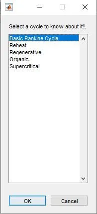
Fig.3: Menu to know about Rankine cycle

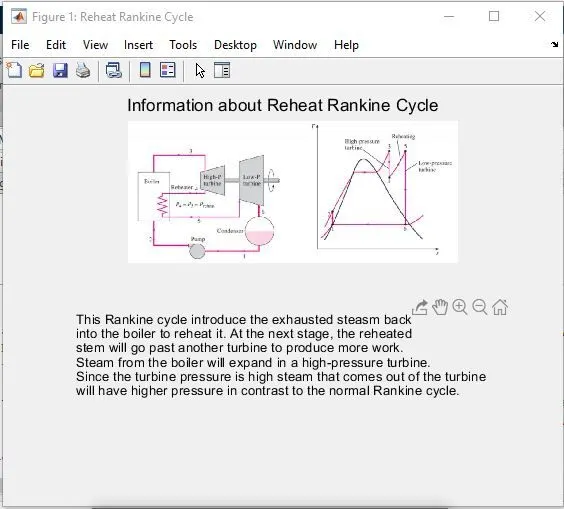
Fig.4: Information about Selected cycle

A pause of 5 seconds is given before going to the next step. This Simulator program can only run the Simple Rankine Cycle. So selecting a Yes will proceed further(displays Success dialog box) and a no can cause the error dialog box.

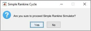
Fig.5: Conformation to proceed to Simple Rankine Simulator

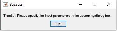
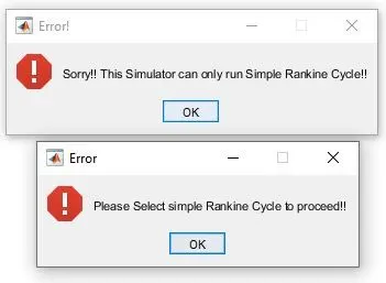
Fig.6: Success Conformation Fig.7: Error Message

After a pause for 5 seconds again, the input prompt pops up to give the input values specified.

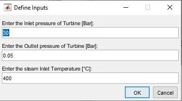
Fig.8: Defining Inputs

The code to display the Outputs of the Rankine Cycle is:

msg = sprintf(['\t\t\t\tRANKINE CYCLE PROCESS  \n'...
    'Process 1-2: Isentropic Expansion Process (Turbine)\n'...
    'Process 2-3: Isobaric Heat Rejection Process (Condenser)\n'...
    'Process 3-4: Isentropic Compression Process (Pump)\n'...
    'Process 4-1: Isobaric Heat Addition Process (Boiler)\n'...
    '\t\t\t\t\nResults of Rankine Cycle \n'...
    '\nAt State Point 1:\t\t\t\t\t\t\t\t\t\n'...
    'Pressure at State 1 = %10f [Bar]\t\t\t\t\n',...
    'Temp. at State 1 = %10f [°C]\t\t\t\t\t\n', ...
    'Entropy at State 1 = %10f [KJ/Kg-K]\t\t\t\n', ...
    'Enthalpy at State 1 = %10f [KJ/K]\t\t\t\n', ...
    '\nAt State Point 2:\n'...
    'Pressure at State 2 = %10f [Bar]\n',...
    'Temp. at State 2 = %10f [°C]\n', ...
    'Entropy at State 2 = %10f [KJ/Kg-K]\n', ...
    'Enthalpy at State 2 = %10f [KJ/K]\n', ...
    '\nAt State Point 3:\t\t\t\t\t\t\t\t\t\n'...
    'Pressure at State 3 = %10f [Bar]\t\t\t\t\n',...
    'Temp. at State 3 = %10f [°C]\t\t\t\t\t\n', ...
    'Entropy at State 3 = %10f [KJ/Kg-K]\t\t\t\n', ...
    'Enthalpy at State 3 = %10f [KJ/K]\t\t\t\t\n', ...
    '\nAt State Point 4:\n'...
    'Pressure at State 4 = %10f [Bar]\n',...
    'Temp. at State 4 = %10f [°C]\n', ...
    'Entropy at State 4 = %10f [KJ/Kg-K]\n', ...
    'Enthalpy at State 4 = %10f [KJ/K]\n', ...
    '\nOther Parameters:\n'...
    'Work done by Turbine = %10f [KJ/Kg]\n', ...
    'Work done by Pump = %10f [KJ/Kg]\n', ...
    'Net Work done (W_Net) = %10f [KJ/Kg]\n', ...
    'Thermal Efficiency(T_eff) = %10f [%%]\n', ...
    'Back Work Ratio(BWR) = %10f [No Unit]\n'],...
    P_1, P_2, T_1, T_2, S_1, S_2, H_1, H_2, P_3, P_4, T_3, T_4, S_3, S_4, H_3, H_4, W_T, W_P, W_Net, Th_eff, BWR);
msgbox(msg,'Rankine Output')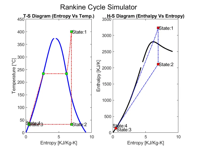

Fig.9: T-S and H-S diagram of Simple Rankine Cycle

For the results msgbox option is used to display it in the order.

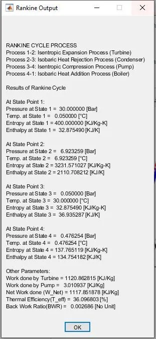
Fig.10: Results of the Simulator

IMPORTANT NOTE:

As there are images attached for the information content of the Rankine cycle. It is necessary to have all the images used in the code as well as the MATLAB function programs to run the simulator without errors.

Rank_try.m - Main file to run the simulator
Simulator_exp.m - Information containing Rankine Cycle types
display_ans_Rankine.m - To display result in command window and write in a new text file
Mok_try.m - To display result in message box

Image Files