Week 3 - Solving second order ODEs
Objective:
Second-order Ordinary Differential Equations (ODE) play an important role in finding solutions for most engineering problems. In this report, we will discuss finding the position of the ball in the pendulum using ODE. The found solution is implemented in MATLAB and visualized as a video output.
A Simple Pendulum:
By Newton's Second Law for rotational systems, the equation of motion of the pendulum is given by,
`frac{d^2theta}{dt^2}+frac{b}{m}*frac{d theta}{dt}+frac{g}{l}*sin theta = 0.`
where,
`theta` - Angular displacement of the pendulum
b - damping co-efficient
m - Mass of the ball in Kg
g - acceleration due to gravity in `m^2/s`
l - Length of the connecting rod in m
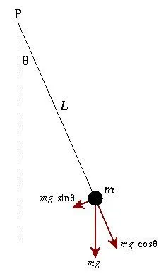
Fig.1: Oscillation of a Simple Pendulum
The above equation was implemented in MATLAB as follows
clear all;
clc;

% Pendulum data
b = 0.05; % Damping Co-efficient
g = 9.81; % [m/s^2] Gravity
L = 1;    % [m] length of rod
m = 0.1;  % [Kg] Mass of ball

% Initial Conditions
T_0 = [0, 3]; % [m m^2] [Initial_displacement Initial_velocity]

% Time Stamps
del_T = 0:0.1:20; % [sec] Time steps for 20 secs with stepsize 0.1

% Solver ODE
% Time and 2 column vector are Outputs using ODE45 command
[Time, Output] = ode45(@(Time,theta)sec_fn_ode(Time,theta,b,g,L,m),del_T,T_0);

%% Plot for Time Vs (Displacement and Velocity)
figure('Name','SHM of Pendulum')
plot(Time,Output(:,1));hold on
plot(Time,Output(:,2));
legend('Displacement [m]','Velocity [m^2]')
xlabel('Time in secs')
ylabel('Parameters of Pendulum')
hold off

%% Video
figure('Name','Pendulum Oscillation')
cla reset
hold on
set(gca,'XTick',[], 'YTick', []) % To remove the numbers for video plot
%clf
%% Plot for the bricks
L=5; % 5 rows in Y-axis
B=20; % 20 blocks in X-axis
C=rand(L,B);
% creating rectangle shape figures
xrec=[-5.6 -4.8 -4.8 -5.6 -5.6 ]; % x-coordinates of the vertices
xrec_even=[-5.2 -4.4 -4.4 -5.2 -5.2 ];
yrec=[0.2 0.2 0.4 0.4 0.2]; % y-coordinates of the vertices
% Using for loop and patch command to fill the shapes
for p=1:B
    j=p-1;
    for k=1:L
        m=k-1;
        if k == 1
            patch((xrec_even+mod(k,1))+0.8*j,(yrec*0.5)+0.2*m,[0.25,0.25,0.25])
        end
        if mod(k,2)== 0
            patch((xrec_even+mod(k,1))+0.8*j,yrec+0.2*m,[0.75,0.75,0.75]); % make a rectangle(brick)
        else
            patch((xrec+mod(k,1))+0.8*j,yrec+0.2*m,[0.5,0.5,0.5]); % if else command is used to create an offset to the brick in the next rows
        end
    end
end
axis([-5 6 -8 10])

%% Plot mid dashed line
plot(zeros(1,101),(-50:1:50),'--','color','k','linewidth',1.5)

% Initializing variables inside the loop
S=0;
ck =1;
% Loop for the animation
for i = 1:1:length(del_T)

    theta = Output(i);
    X_0 = cos(Output(1,1)-(pi/2));
    Y_0 = 0;
    X(i) = L * cos(Output(i,1)-(pi/2));
    Y(i) = L * sin(Output(i,1)-(pi/2));

    %% Plot for Fixed Pin
    AA = plot(0,0,'Marker','o','MarkerSize',10,'MarkerEdgeColor','k','MarkerFaceColor','k'); % plots pin

    %% Plot for Rod(CHANGE POSITION)
    BB = plot([0 X(i)],[0 Y(i)],'b','LineWidth',4);


    %% Plot for sphere(CHANGE POSITION)
    CC = plot(X(i),Y(i),'Marker','o','MarkerSize',25,'MarkerFaceColor','m','MarkerEdgeColor','k'); % plots bob
    DD = plot(X(i),Y(i),'Marker','.','MarkerFaceColor','k','MarkerEdgeColor','k'); % Dot Path for the ball
    if X(i)>S
        EE = plot(X(i),Y(i),'Marker','>','MarkerFaceColor','g','MarkerEdgeColor','k'); % green arrow for clockwise direction
    else
        EE = plot(X(i),Y(i),'Marker','<','MarkerFaceColor','r','MarkerEdgeColor','k'); % red arrow for clockwise direction
    end

    % Saving the plots as frames
    H(ck)= getframe(gcf);
    ck = ck+1;

    % Visiblity control for plots
    set(BB,'Visible','off') % hold off the rod plot and updates the new position in next loop
    set(CC,'Visible','off') % hold off the Sphere plot and updates the new position in next loop
    set(EE,'Visible','off') % hold off the Arrow plot and updates the new position in next loop

    S = X(i) % declaration to run if-else loop for arrows

    % annotation for video
    annotation('textbox',[.3 .5 .3 .3],'String','Oscillation of a Simple Pendulum','FitBoxToText','on');
end

movie(H)
ani = VideoWriter('ODE.avi','Uncompressed AVI'); % writing the video in the name "ODE.avi"
ani.FrameRate=8; % Control the framerate of video
open(ani)
writeVideo(ani,H)
close(ani)
The steps of the code are explained as comments in the editor.
A secondary call-back function was used in the code to execute the ODE function. The code for the call back function "sec_fn_ode.m" is
function [dTheta_dt] = sec_fn_ode(Time,theta,b,g,l,m)

theta1 = theta(1);
theta2 = theta(2);

dTheta1_dt = theta2; % First ODE
dTheta2_dt = -((b/m)*theta2) - ((g/l) * sin(theta1)); % Second ODE

dTheta_dt = [dTheta1_dt; dTheta2_dt]; % Combining both ODE's

end
The entire program was set to run for 20 secs and the output graph of the time versus other parameters like displacement and velocity was found.
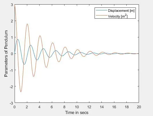
Fig.2: Time Vs (Displacement and Velocity)
Link for the Video File:
Problems while coding:
- Hold on command in the plot was very important to hold the other images like the bricks, dotted centerline, and the pin to hold the pendulum. Due to the hold on command, the previous outputs of the ball, rod, and arrow were also seen. To avoid this, visibility off option in the plot command was used to always display only the updated image of the plot even though hold command was used.
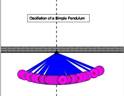
Fig.3: Error during execution
Conclusion:
Thus the MATLAB program for implementing an ordinary differential equation was explained. The output plots were stitched into a single video for a better understanding of the results.