Aim

To create a MATLAB-Simscape physical model for an all-terrain vehicle (ATV) and carry out a system-level simulation at various conditions.

Objective

1. To Simulate vehicle from the start without any external actuation on a flat terrain.
2. To Simulate vehicle model on 1 degree (or pi / 180 rad) downward slope without head wind.
3. To Simulate vehicle model on 1 degree (or pi / 180 rad) downward slope with 2m/s head wind.
4. To Simulate the model by adding variable terrain.
5. To Incorporate Braking system, clutch, 3-speed gear transmission and ‘’generic combustion engine’ block in the model.
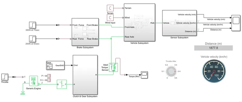
6. To simulate the model by applying 300 N force via front brake at 75 sec and 200N force via rear brake at 50 sec. Also, shift the gear from low to mid to high gear at an equal interval of 10seconds. Note its effect on vehicle torque, speed, tyre slip and normal force.

Introduction

An all-terrain vehicle (ATV) also known as quad bike, or simply a quad is a light utility vehicle (LUV) that travels on low-pressure tires, with a seat that is straddled by the operator, along with handlebars for steering control. It is designed to handle a wider variety of terrain than most other vehicles. The rider sits on and operates these vehicles like a motorcycle, but the extra wheels give more stability at slower speeds. Although most are equipped with three or four wheels, six-wheel models exist for specialized applications.

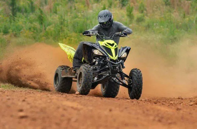
In this project a block model of an ATV actuated by a combustion engine will be built and simulation will be carried out. The input data values for various components like engine, tires, braking system etc are either taken from ‘Mathworks’ website or default values are used. Finally, various output parameters of the vehicle will be taken into account to measure the vehicle behaviour.

Methodology

For this project MATLAB/Simulink software is used. MATLAB is a High-level language using which we can write a programme, solve numerical problems, analyse and visualize data. Whereas Simulink is a Block diagram environment within MATLAB where we can model and simulate a system, perform dynamic analysis and analyse the data. Simscape extends Simulink with libraries for modelling and simulating multidomain physical systems. With Simscape we create the model using the physical network method where deriving system level equations are not required.

When simulating simscape model certain Simulink solvers are recommended. These are ode15s and ode23t for variable step simulation. And for fixed step simulation, ode14x.

Every physical network in a simscape model should have a solver configuration block theses are used to set solver parameters per network. If a simscape model have more physical network then it will have more than one solver configuration block.

Simscape Model & Blocks used

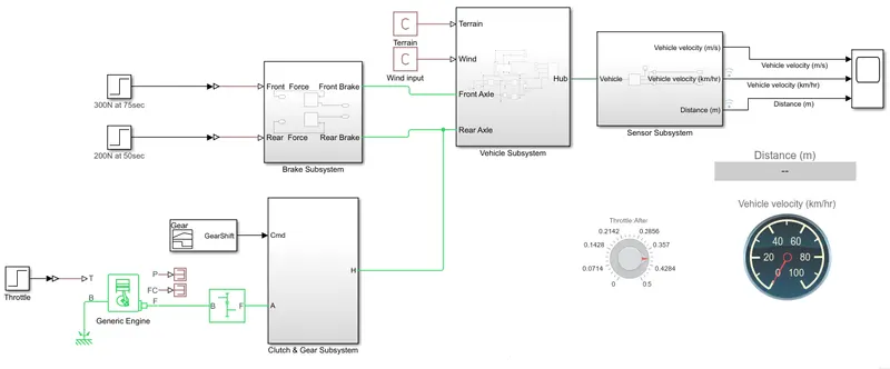
Final ATV Simscape Model:

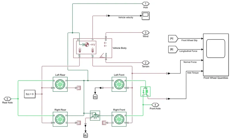
• Vehicle Subsystem

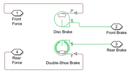
• Brake Subsystem

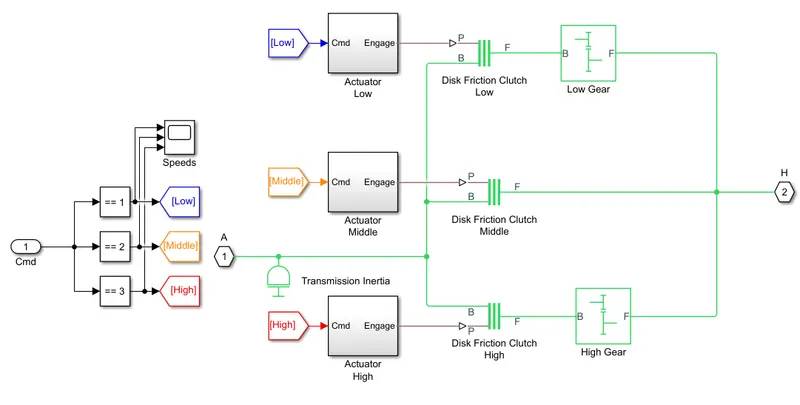
• Clutche and Gear Subsystem

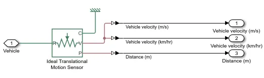
• Sensor Subsystem

Some essential Blocks Used:

• Vehicle Body Block

It allows us to model the longitudinal dynamics of the vehicle. Lateral forces associated with steering, inclination or other external forces is not accounted for in the block equations. It has several ports, ‘V’ represents longitudinal velocity of the vehicle. The front and rear normal forces i.e., load on the wheel at port ‘NF’ & ‘NR’. The horizontal motion of the vehicle is represented by the port ‘H’.

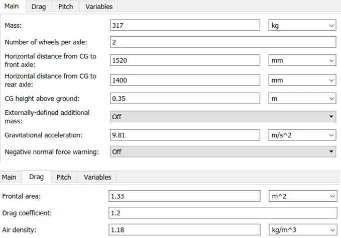
Block Parameters:

• Tire

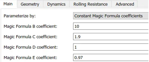
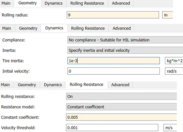
Magic formula is a popular way to model tires. At port ‘N’ we specify verticle load, the block reports the developed slip at port ‘S’, wheel axle rotaion is represented by port ‘A’ & the wheel axle horizontal motion is represented by port ‘H’.

Specifing the variables:

Making port connections:

Connect the ‘Normal force port (N) of the ‘tire’ block to the front and rear normal force port (NF & NR) of the ‘vehicle body’ block. This will define verticle downward load and also specify one tire as front wheel and other as rear.

Connect ‘H’ port of vehicle body to ‘H’ port of the wheels. Since, Connection ‘H’ is the mechanical translational conserving port for the wheel hub through which the thrust developed by the tire is applied to the vehicle.

Next, component is the rotational component of the tire itself. This is obtained at ‘A’ port of the tire.

Port ‘S’ are used to measure wheel slip & can be connected to the ‘Scope’.

• Generic Engine Block

Generic engine block has several ports. A throttle input signal port ‘T’ signifies normalised engine torque. Its value varies b/w 0 & 1.

Based on this throttle, the engine reports the Power and fuel consumption rate through the port ‘P’ and ‘FC’. ‘B’ and ‘F’ are rotational ports that specify base and follower shaft.

The Engine block is parametrised after loading the Torque-RPM data file in MATLAB. And then specifying the engine block values as given below.

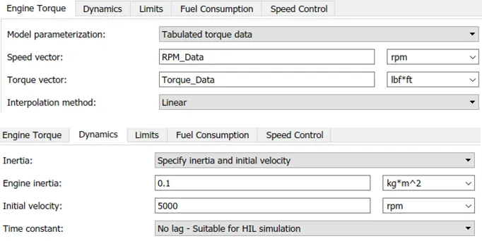
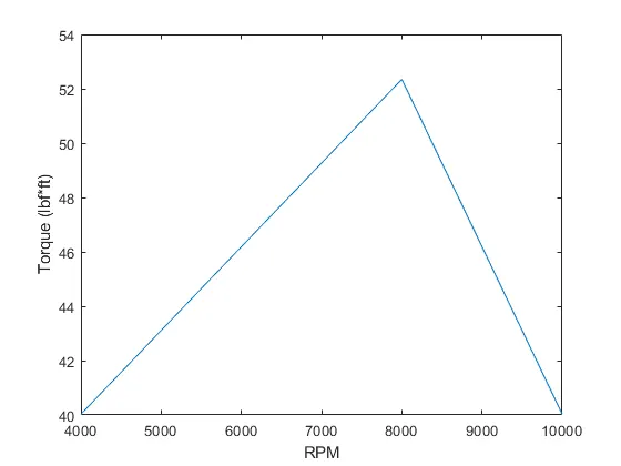
Following is the plot of Torque-RPM data use for engine block:

Results & Discussion

1. Starting vehicle from the start without any external actuation on a flat terrain.

• Vehicle Model:

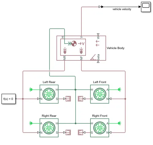
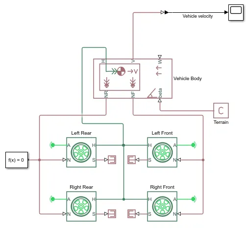
For this case, vehicle is not powered by any external source for its movement. The front and the rear axles are completely independent of each other and are free to rotate without any resistance baring whatever the tire has. To implement this condition, we will add ‘Rotational free end block’ at port ‘A’.

• Velocity Plot:

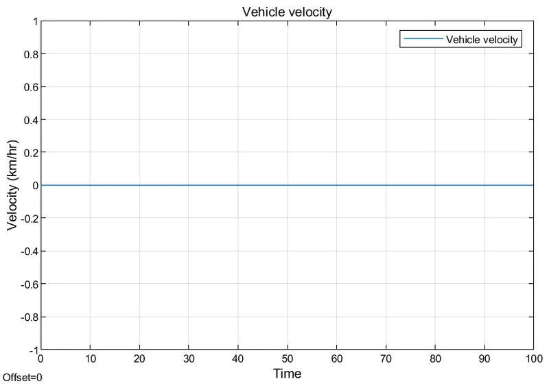
When there is no external actuating force to move the vehicle and the terrain in flat the vehicle velocity remains zero.

2. Vehicle model on 1 degree (or pi / 180 rad) downward slope without head wind.

• Vehicle Model:

• Velocity Plot:

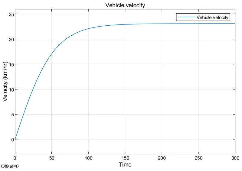
For this condition, the simulation time has been increased to 300 seconds to see when will the vehicle attains stedy state velocity. The vehicle attains stedy state velocity at around 200 seconds.

Due to downward inclination, the vehicle accelerates and its velocty increases from zero to a stedy state velocity of 22km/hr.

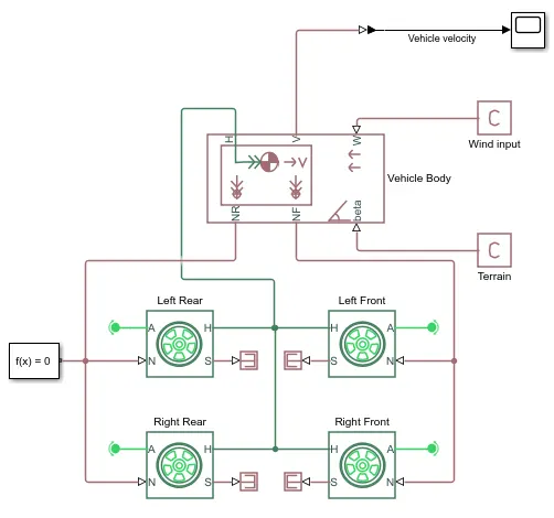
3. Vehicle model on 1 degree (or pi / 180 rad) downward slope with a head wind of 2m/s.

• Vehicle Model:

• Velocity Plot:

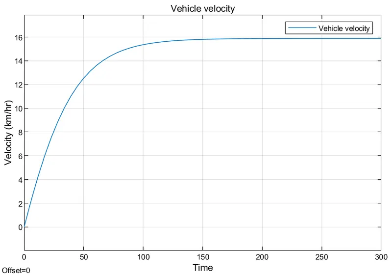
Vehicle reaches a steady speed after about 200 seconds. This is due to the wind, slope and rolling resistance of the tire in the model.

The vehicle velocity has reduced in comparison to the previous case. Now the resultant steady state velocity of the vehicle is about 16 km/hr. This reduction is due to opposing wind, drag due to frontal area of the vehicle and the rolling resistance of the tire.

4. Adding Variable terrain in our model.

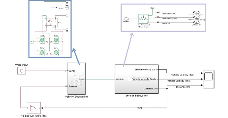
In practice terrain could be non-uniform which can be imported into MATLAB from an external file. To specify non uniform terrain, we will specify the gradient of the terrain based on the distance i.e. odometer measurement. This relationship will be implemented using a lookup table.

• Plot of variable terrain data used is shown below:

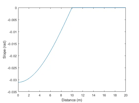
As seen from the plot, the slope of downward inclination gradually reduces eventually become zero.

• Vehicle Model:

• Velocity and Distance Plot:

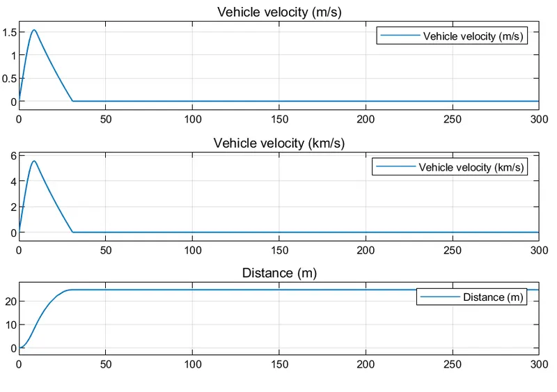
From the velocity plot it is clear that the the vehicle accelerates initially due to inclination, velocity reaches its peak, finally the velocity reduces as the slope reduces and eventually the surface becomes flat and the vehicle becomes zero.

Incorporating Braking System in our model.

• Vehicle Model:

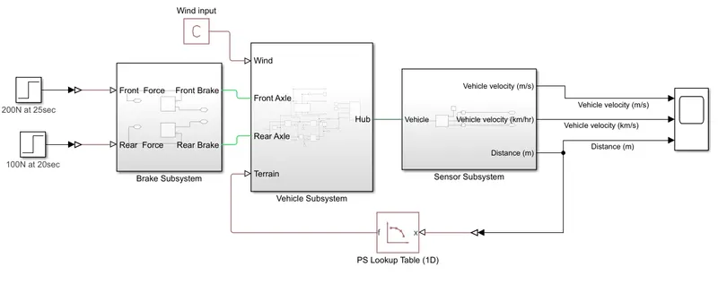
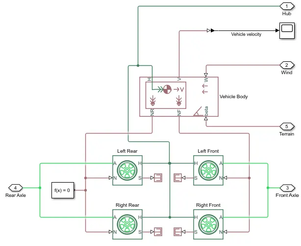
To incorporate Brakes in the vehicle, we need to access the vehicle subsystem and delete ‘rotational free ends’ from the tires and insert output ports for the brakes as shown.

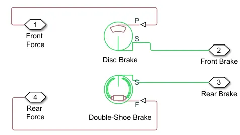
Inside Brake subsystem, Disk brake for front tyres and shoe brake for rear tyres are used.

• Velocity and Distance plot:

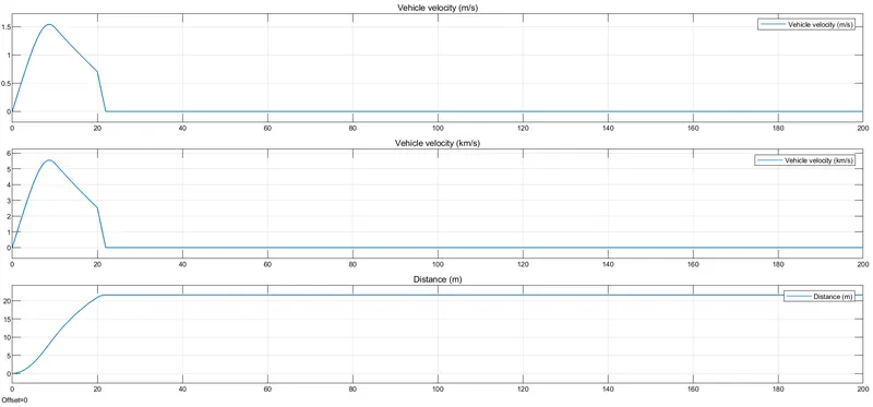
Here, the motion of the vehicle is due to gravity as it decent on the slope. After running the simulation we can see, due to application of rear brake at 20 seconds and front brake at 25 seconds, the vehicle has deacellerated faster.

6. Simulation with 3-speed transmission and using actuating source as an engine block.

For this case, 300 N force will be applied via front brake at 75 sec and 200 N force via rear brake at 50 sec.

From 0- 10 sec low gears (gear ratio = 3:2) will be engaged. Form 10 -20 sec mid gear (gear ratio = 1:1) will be engaged. From 20 – 30 sec high gear (gear ratio = 2:3) will be engaged.

Effect on vehicle torque, speed, tyre slip and normal force will be noted.

• Vehicle Model:

• Velocity and Distance plot:

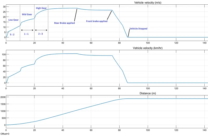
We can clearly see the effect of gear shift of the plot. With successive change in gear the velocity of the vehicle increases and reaches a steady state velocity of 100 km/hr at around 40 sec.

The low gear with high gear ratio, results in higher acceleration. Whereas high gear provides high speed with relatively lower acceleration and hence lower torque.

The velocity reduces after the application of the rear brake at 50 sec. The speed of the vehicle was high enough to overcome the resistance provided by the rear brake application. But after the application of the front brake at 75 sec, the vehicle speed reduces drastically, since both rear and front gears are engaged. The vehicle comes to a halt at around 85 seconds.

• Torque Plot:

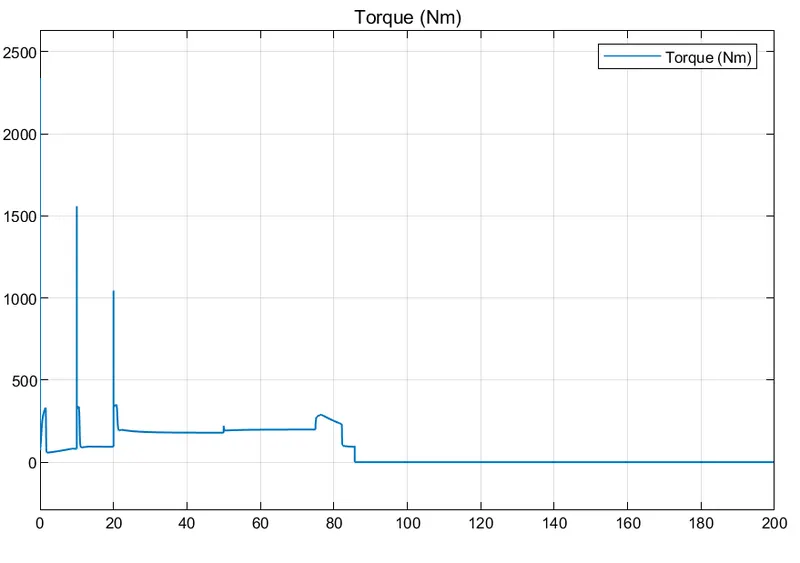
From the above plot we can see the effect of acceleration and brake application on torque. The value of torque reduces at higher transmission. This is because at high gears the velocity increases with decrease in acceleration and torque.

We can also see, increase in engine torque with the application of brake at 50sec and 75 sec.

• Front wheel output parameters:

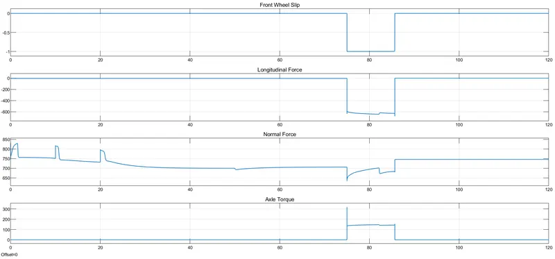
The plot shows forces on front wheels due to the application of brakes and gear shift. At 75 sec when front brakes are applied the front tires slips as well as the longitudinal force on the front tire wheel hub also increases. From the ‘Normal force’ plot we can see the effect of gear shift on the front wheels. The ‘Axle Torque’ plot shows increase in torque on front wheel when the front brakes are applied.

Conclusion

In this project a 3-speed manual transmission ATV model was built using MATLAB-Simulink block diagram. Various components such as braking system, clutch, gear transmission, speedometer, odometer etc. were incorporated in the model. The effect on the vehicle was studied in non-uniform terrain with and without head wind. Finally, the vehicle was actuated using a generic engine and the effect of gear shift brake actuation was noted on the front wheel, torque and vehicle speed.

Reference List

Mathworks.com

Howstuffsworks.com

wikipedia.org