Project 2 Thermal modeling of battery pack

2.Objective

To analyze temperature and life cycle parameters of the 10 cell series battery pack.

• Connect 10 cells in series analyze the response to a cyclic charge and discharge source.
• Change the ambient temperatures of the battery pack and compare the performances.
• Add the fading parameters of the battery and analyse the performance after each charge/discharge cycles.

3.Simulink Modelling of Battery pack

3.1 Need of Battery Modelling

An accurate forecast of the remaining driving range of an electric vehicle (EV) is crucial to avoid range anxiety. Drivers need to know how much further they would travel before their vehicle batteries require a recharge. In addition, the battery management system should predict when batteries need replacement. The remaining charge calculation must be precise to utilize the battery’s full capability. The state of charge (SOC) of a battery or pack of batteries is analogous to a fuel gauge of a conventional vehicle.

3.2 Battery Modelling

The Battery modeling procedure followed in the MATLAB is explained below. The MATLAB model is available from the library given below.

Battery (Table-Based)

Library:

Simscape / Electrical / Sources

The Battery (Table-Based) block represents a high-fidelity battery model. The block calculates no-load voltage as a function of charge level and optional temperature using lookup tables and includes several modeling options:

• Self-discharge
• Battery fade
• Charge dynamics

The Battery (Table-Based) block has four modeling variants, accessible by right-clicking the block in your block diagram and then selecting the appropriate option from the context menu, under Simscape > Block choices:

• Uninstrumented | No thermal port — Basic model that does not output battery charge level and simulates at a fixed temperature. This modeling variant is the default.
• Uninstrumented | Show thermal port — Model with exposed thermal port. This model does not output internal charge level of the battery.
• Instrumented | No thermal port — Model with exposed charge output port. This model uses a fixed temperature throughout the simulation.
• Instrumented | Show thermal port — Model that lets you output internal charge level of the battery. Both the thermal port and the charge output port are exposed.

The instrumented variants have an extra physical signal port that outputs the internal state of charge. Use this functionality to change load behavior as a function of state of charge, without the complexity of building a charge state estimator.

The thermal port variants expose a thermal port, which represents the battery thermal mass.

The battery equivalent circuit is made up of the fundamental battery model, the self-discharge resistance RSD, the charge dynamics model, and the series resistance R0.

3.3 Battery Modeling Procedure followed by MATLAB

Equivalent circuit modeling is the most common approach for battery numerical analysis. For lithium cells, a one or two RC block model with no parasitic branch is a common choice. It has the advantage of being computationally simple and is easily combined with other methods such as coulomb counting with an OCV / SOC correlation for periodic recalibration during rest.

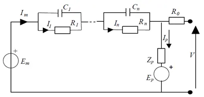
Figure 1: A general equivalent circuit model of an electrochemical cell.

The number of equivalent circuit elements results in a trade-off between fidelity and complexity. The parasitic branch can be neglected for cells with high columbic efficiencies.

Depending on the characteristics of the problem to be analyzed, the number of RC blocks typically ranges from one to two, since larger numbers increase computational effort without significantly improving model accuracy.

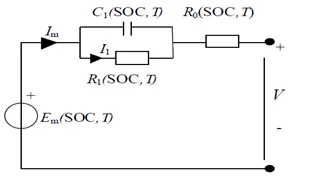
Figure 2: Equivalent circuit of the cell used in this model

• Thermal modeling

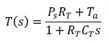
The value of the equivalent circuit components depends on SOC and inner cell temperature. The inner cell temperature is assumed to be uniform, and taken as the average temperature inside the cell. This cell temperature can be computed by solving the heat equation of a homogeneous body exchanging heat with the environment.

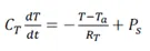
Where C_T = heat capacitance (J m-3 K-1)

T = Inner cell temperature (ºC)

Ta = ambient temperature (ºC)

R_T = convection resistance (W1 m-2 K-1)

Ps = power dissipated inside the cell (W)

Taking Laplace transform we get,

• Cell capacity and state of charge

The cell capacity (extractable charge) depends upon a number of factors, including:

1. average cell discharge current and discharge time
2. Inner cell temperature
3. Value of the end-of-discharge voltage
4. Storage time (self-discharge)
5. Number of charge-discharge cycles that the cell has undergone (aging)

For short periods of time we can restrict the list above to average cell discharge current, discharge time, and inner cell temperature.

Hence, cell capacity,

Assuming the cell to be fully charged at time t=0, the extracted charge, Qe is defined as:

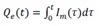
Im = Current in main branch (A)

Then, the state-of-charge (SOC) is:

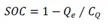
where C_Q is the capacity of the cell at the temperature and discharge current considered. Consequently, any SOC definition should consider the conditions under which a cell is discharged and refer to the particular discharge current and temperature under which the SOC has been evaluated.

• Equivalent circuit model parameters

Each element of the equivalent circuit of Figure 2 is a function of SOC and temperature. Specifically:

R0= R0(SOC,T)

R1=R1(SOC,T)

C1=C1(SOC,T)

Em= Em(SOC,T)

The parameter estimation routine was run for a range of discharge experiments at different temperatures. The results provide two-dimensional look-up tables each of these four equivalent circuit elements.

3.4 MODELING AND SIMULATION

The numerical analysis proposed here consisted of a parameter estimation / validation stage, and a simulation stage. During parameter estimation, a discharge profile was iteratively simulated and its results compared with experimental data. The ECM was created using SimscapeTM blocks and SimscapeTM language. The drawing shown in Figure 4 represented the circuit diagram with a single RC block. Each of the circuit elements was a subsystem consisting of custom electrical blocks, and blocks to calculate the properties of the circuit element.

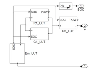
Figure 3: Simscape Equivalent Circuit Model

The resistive circuit elements were modeled as variable resistors, as shown in Figure 4. These were modeled based on Ohm’s Law, though a minimum resistance value was used to prevent the differential equation solver from entering a bad state during parameter estimation or simulation. The real power of the resistive elements was also calculated for later use in simulation of thermal dynamics. The value of the resistance was provided by a lookup table with one or two inputs of SOC and temperature.

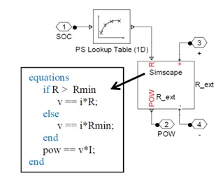
Figure 4: Resistive Circuit Element and Simscape Language

The model was validated using a single 20-minute New European Drive Cycle, which showed cell voltage accuracy within 2%. The model accounts for the inner heat generated in the cell and the corresponding thermal build-up; and predicted the cell voltage and SOC for an arbitrary current profile. The procedure also illustrates a way in which Simscape may be utilized as a numerical tool for modeling electrochemical systems using equivalent circuits, in combination with the parameter estimation functionalities of Simulink Design Optimization.

3.4.1 Modeling Battery Fade

It is generally thought that lithium deposition, electrolyte decomposition, active material dissolution, phase transition inside the insertion electrode materials, and further passive film formation on the electrode and current collectors can affect up to different degrees the capacity fade of lithium-ion batteries. Quantifying these degradation processes will not only help to improve the predictive capability of battery models but also help to elucidate the mechanism of capacity fade.

Three major causes of capacity fade including the loss of secondary material, the loss of primary material and the difference of rate capability were quantified. In each case the loss of the secondary material dominated the capacity fade of the whole cell. However, unlike the 1C-discharge-ratecycled battery, the limiting secondary material the in 3Cdischarge- rate-cycled cell was carbon. The capacity loss due to the carbon electrode material alone was 10.6% compared with the 16.9% capacity fade of the whole cell. Such a fast capacity fade for the carbon material is correlated with the increase of the internal resistance. Fitting impedance spectra for the carbon half-cell quantitatively showed that the resistance of the surface film and the resistance of the bulk carbon material increase faster for high-rate-discharged cells than for normal-rate-discharged cells.

The battery fade is modeled in MATLAB as follows.

• No load voltage change

The no load voltage across fundamental battery is modeled using the equation below.

V_0,fade = V₀ ( 1+ (dV₀ * n / 100*N))

Where,

N is the reference number of discharge cycles over which we specify percent change of various battery parameters.

dV₀ is the change in no load voltage after N discharge cycles.

• Battery Capacity change

Q_nom,fade = Q_nom (1+ d_AH* sqrt(n/N)/100)

Where, Q_nom is the rating of the battery

d_AH is the change in AH rating after N cycles

• Change in Resistance

R_i,fade = R_i (1+ (d_Ri * sqrt (n/N)/100))

Where, R_i is the series resistance of the battery

d_Ri is the change in series resistance after N cycles

3.5 Selection of values for Battery pack

All the cell parameters depend upon Temperature and SOC and the values of them are given below.

Temperature_LUT(1*3) = [278.15   293.15    313.15]

SOC_LUT(7*1) =  0

                              0.1

                              0.25

                              0.50

                              0.75

                              0.90

                              1

The other parameters like No-load voltage(Em_LUT), Terminal resistance (R0_LUT), First polarization resistance (R1_LUT), and time constant(TC) are extracted from MATLAB example[5].

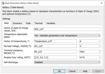
Figure 5: Main battery parameters

Since battery model is table based with temperature dependent, all the values have entered depending upon temperature and SOC.

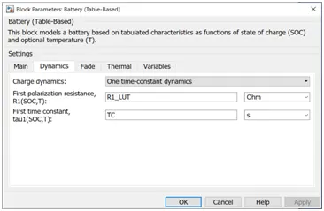
Figure 6: Dynamics of battery

For simplicity of analysis, only one time constant has considered.

4. Output Analysis

4.1 Temperature Analysis

The battery performance parameters like Voltage, SOC has to be analysed at different temperatures.

Figure 7 shows the battery pack model with 10 cells connected in series. All these cells are connected such that it can transfer heat by conduction and convection. The ambient temperature can be changed to different values to analyse the battery pack performance at different temperatures.

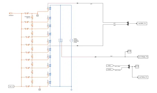
Figure 7: Simulink model of 10 cell connected in series for temperature analysis

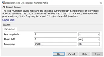
Figure 8: Cyclic charge/discharge profile

An AC source has been connected to analyse the cyclic charge and discharge performance. The positive cycle will charge the battery and negative cycle will discharge the battery. Peak Amplitude has given 3A so that the charging/ discharging doesn’t go beyond 1C rate.

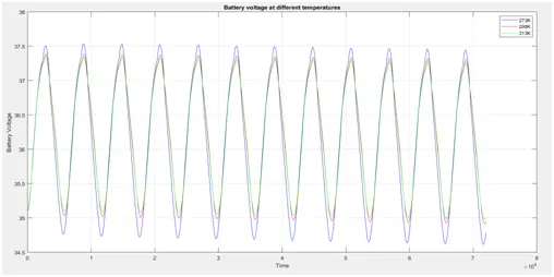
Figure 9: Terminal voltage of battery pack at different temperatures

For the comparison to be more specific, simulation ran 3 times by changing the ambient temperature values 273K (0 degC), 298K (25 degC), 313K (40 degC). These output results stored in workspace in out_T0, out_T1, out_T2 respectively as shown in figure 10.

The terminal voltage of the battery pack has been plotted in figure 9. From the above plot we can see that battery pack voltage will be maximum at 273K (0 degC). As the temperature increases, the battery pack voltage reduces.

The performance of the battery at 273K is such that it is going to peak voltage and lowest voltage. From SOC plot in figure 11, we can see that at zero SOC, terminal voltage falls below the cut off voltage which is not desirable.

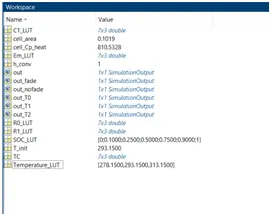
Figure 10: Workspace variables

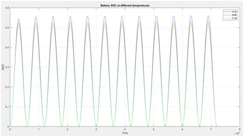
Figure 11: SOC of Cell1 at different ambient temperatures

For comparison purpose only SOC of cell1 has considered. Since the cells are connected in series, there will be some difference in charging/ discharging of each cell.

In figure12, cell 1 temperature plotted at different ambient temperatures. We can see that after 10,000sec, the temperatures are settling to ambient temperature.

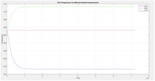
Figure 12: Temperature of cell1 at different ambient temperatures

4.2 Life cycle Analysis

Figure 13 shows the Simulink model of battery pack for lifecycle analysis is shown below. From [2] and [3], we know that the terminal voltage and capacity of the battery will decrease and internal resistance will increase after specified number of cycles.

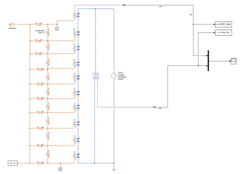
Figure 13: Simulink model of battery pack to analyse battery fading

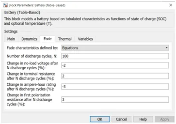
Figure 14: Fade parameters of battery

For the fade data I’ve just given some arbitrary values for the purpose of simulation analysis. In actual case, battery fading happens after 2000-5000 cycles depending upon battery type. But to analyse the performance in simulation, 100 cycles have given.

1. Change in no-load voltage = -2% (This indicates that the no load voltage will reduce 2% after N cycles)
2. Change in terminal resistance = 2% (The terminal resistance will increase by 2%)
3. Change in AH rating = -3% (Ampere hour decrease by 3% after N cycles)
4. Change in first polarization resistance = 3% (First polarization resistance increase by 3%

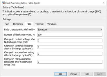
Figure 15: Making the fade parameters to zero to compare performance

For comparison of analysis, simulation ran 2 times and saved the data in ‘out_fade’ and ‘out_nofade’ variables. In first simulation, all the cells are entered with fade parameters as shown in figure 14 and saved the output in out_fade variable in WS. In second simulation, all the cells fade parameters made to zero as shown in figure 15 and saved the output in out_nofade variable in WS.

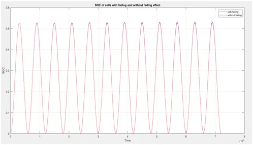
Figure 16: SOC of cell1 comparison plot

In figure 16, we can see that the SOC is a bit higher for battery with fading effect(Blue plot) that without fading plot (Pink plot).

This is due to the deterioration of capacity of the battery we added in fade parameters. As the life cycle increases, battery maximum charge and maximum discharge varies as shown in the above plot.

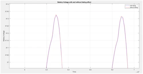
Figure 17: Terminal voltage of battery pack by adding fading parameters and removing it

To obtain the terminal voltage of battery pack without fading effect, all the fading parameters set to zero and the output of simulation was saved in WS.

In figure 17, terminal voltage of the battery pack decreases as the cycles proceed. This is because of the fading effect. For battery without fading effect, terminal voltage remains the same.

5.Conclusion

MATLAB library model parameters were evaluated for its life cycle and thermal effects parameters. A battery pack with 10 cells connected in series also made with a source of charging and discharging cycle.

The thermal effects of battery pack at different ambient temperatures for cycling charging/discharging has been analysed and plotted. The life cycle performance also evaluated for individual cells and overall battery pack.

6.Future Scope

In this model, individual cells were connected in series to make the battery pack. The thermal and life cycle performance of individual cells are different from battery pack.

In future we can consider the battery pack parameters to analyse the performance.

Also there are different associated components that contribute the temperature increase such as charger, connectors, wire resistances etc. In future, all these parameters have to be considered while analysing thermal behaviour.