Project - Data Handling and Interpolation

AIM:

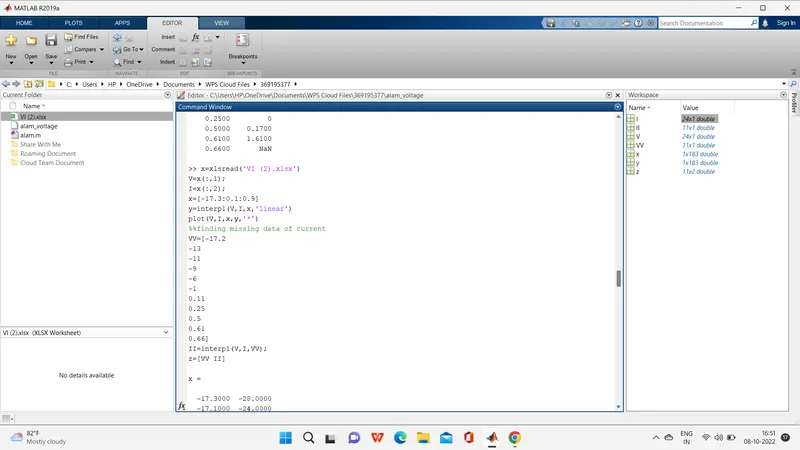
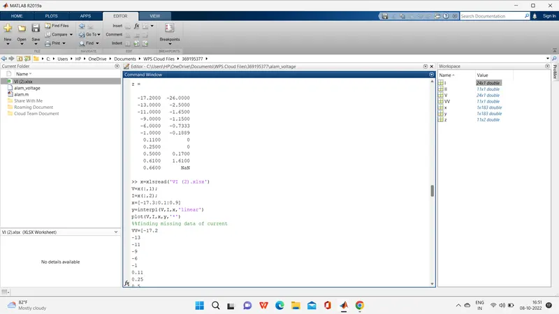
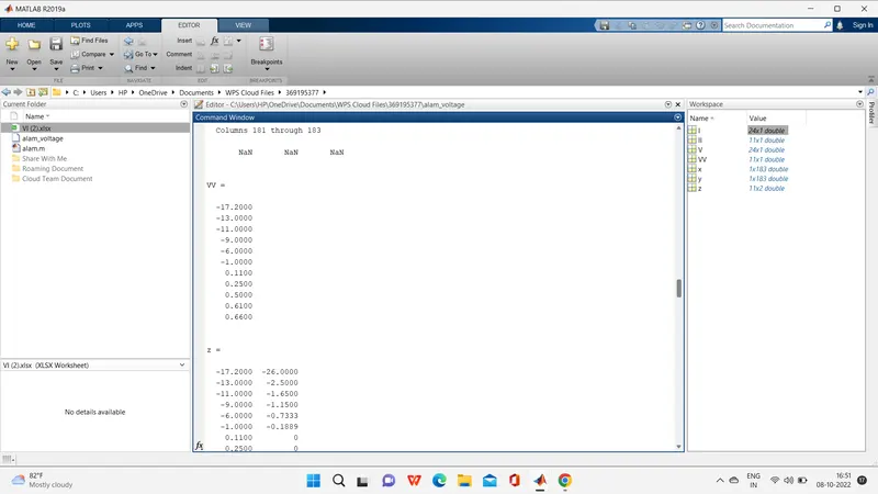
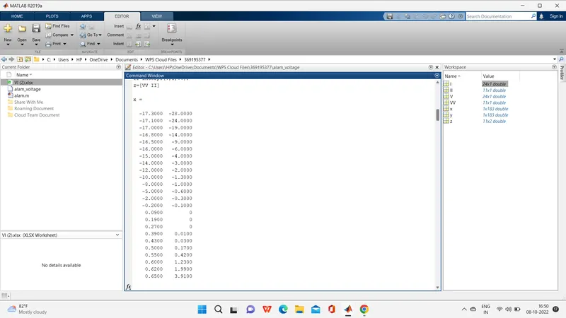
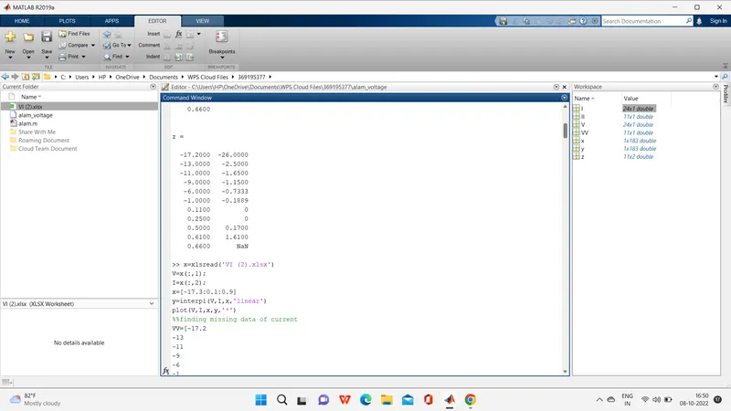
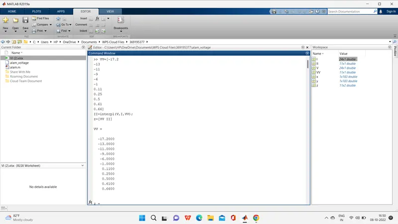
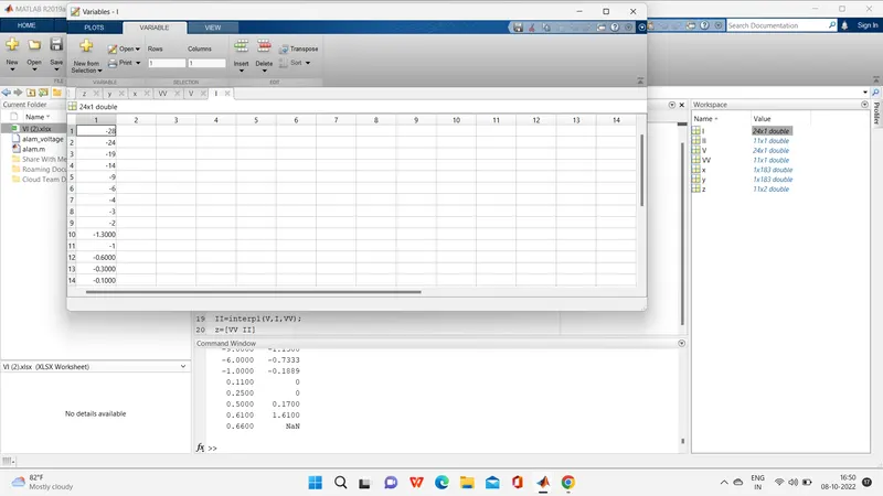
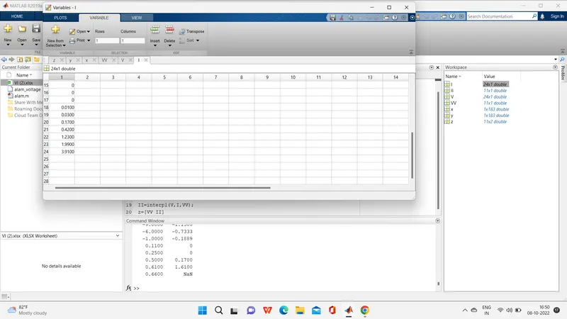
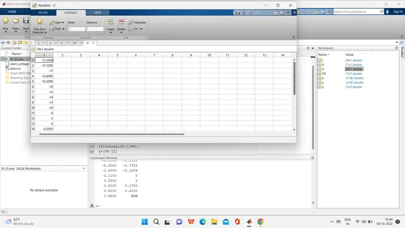
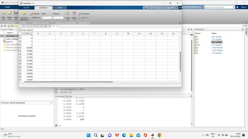
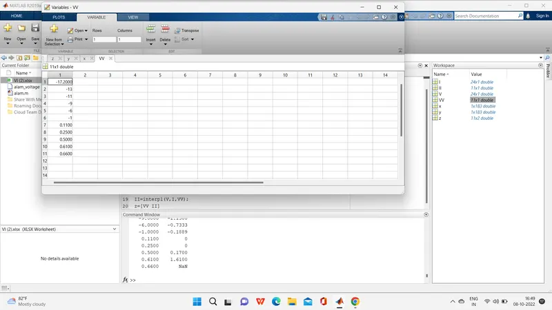
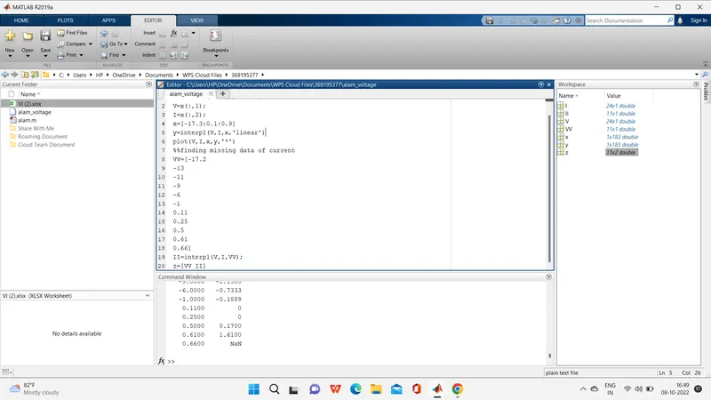
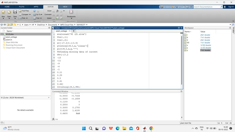
• In this project, we are reading the excel file into the MATLAB program.
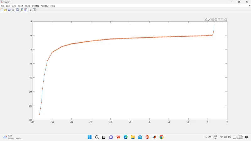
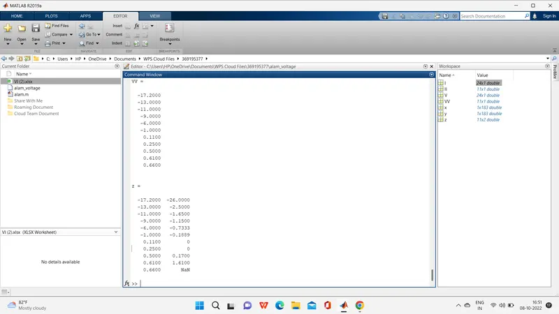
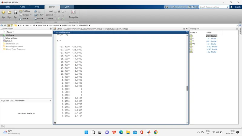
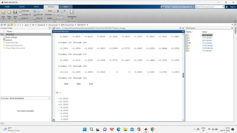
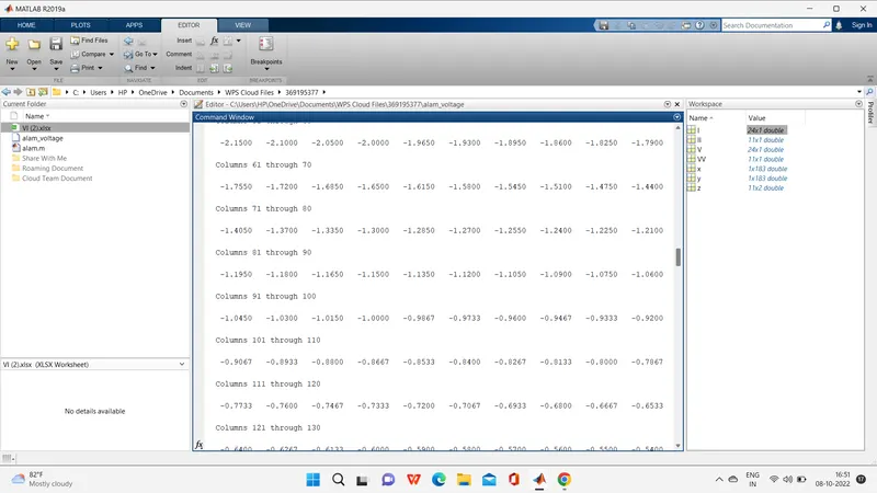
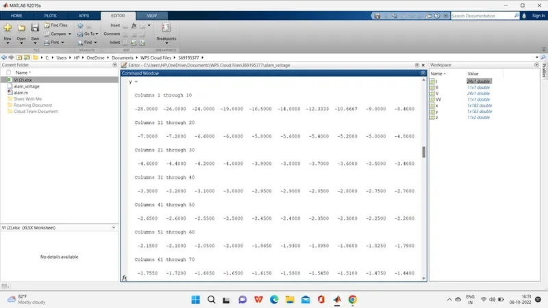
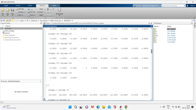
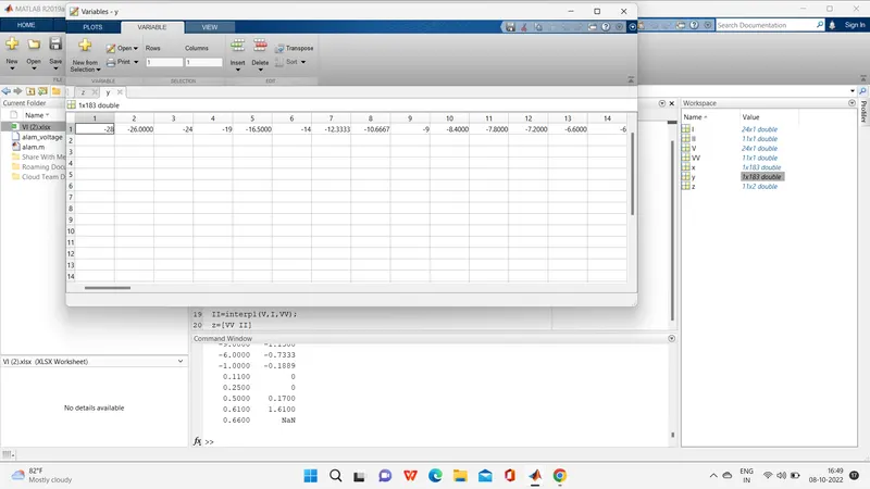
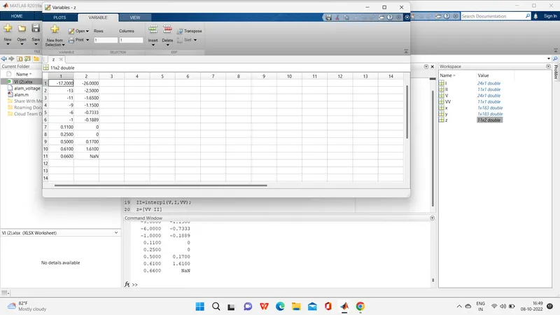
• perform the interpolation in the range of -17.3:0.1:0.9
• Generate the interactive plot for the interpolated data and store them in a text file.

What is interpolation?

Interpolation is a method of fitting the data points to represent the value of a function. It has various applications in engineering and science, that are used to construct new data points within the range of a discrete data set of known data points or can be used for determining a formula of the function that will pass from the given set of points (x, y).

Types of interpolation methods are:

1. Linear interpolation
2. Nearest neighbor interpolation or Piecewise constant interpolation
3. Polynomial interpolation
4. Spline interpolation
5. Mimetic interpolation
6. Cubic Spline Interpolation

1. Linear interpolation:

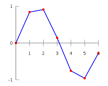
A linear interpolation is a form of interpolation, which involves the generation of new values based on an existing set of values. Linear interpolation is achieved by geometrically rendering a straight line between two adjacent points on a graph or plane. All points on the line other than the original two can be considered interpolated values.

Linear Interpolation Formula

The formula to calculate linear interpolation is:

Linear Interpolation(y) = y1+(x−x1) (y2−y1) (x2−x1) y1+(x−x1) (y2−y1) (x2−x1)

were,

• x1x1 and y1y1 are the first coordinates
• x2x2 and y2y2 are the second coordinates
• x is the point to perform the interpolation
• y is the interpolated value

2. Nearest neighbor interpolation or Piecewise constant interpolation

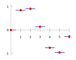
Interpolation is the problem of approximating the value of a function for a non-given point in some space when given the value of that function in points around (neighboring) that point. The nearest neighbor algorithm selects the value of the nearest point and does not consider the values of neighboring points at all, yielding a piecewise-constant interpolant.

3. Polynomial interpolation

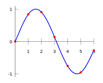
Polynomial interpolation is a method of estimating values between known data points. When graphical data contains a gap, but data is available on either side of the gap or at a few specific points within the gap, an estimate of values within the gap can be made by interpolation.

4. Spline interpolation

Spline interpolation similar to the Polynomial interpolation x’ uses low-degree polynomials in each of the intervals and chooses the polynomial pieces such that they fit smoothly together. The resulting function is called a spline.

5. Mimetic interpolation

mimetic interpolation is a method for interpolating differential forms. In contrast to other interpolation methods, which estimate a field at a location given its values on neighboring points, mimetic interpolation estimates the field's k{\displaystyle k} Kk-form given the field's projection on neighboring grid elements. The grid elements can be grid points as well as cell edges or faces, depending on k=0,1,2, 3…{\displaystyle k=0,1,2,\cdots }.

Mimetic interpolation is particularly relevant in the context of vector and pseudo-vector fields as the method conserves line integrals and fluxes, respectively

6. Cubic Spline Interpolation:

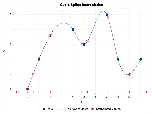
Cubic spline interpolation is a special case for Spline interpolation that is used very often to avoid the problem of Runge's phenomenon. This method gives an interpolating polynomial that is smoother and has smaller errors than some other interpolating polynomials such as Lagrange polynomial and Newton polynomial.