Project 2 - Rankine cycle Simulator

1. AIM :

To create a Rankine cycle simulator and to find out the thermodynamic properties at each state.

2. GOVERNING EQUATIONS :

• 1-2 Isentropic expansion in a turbine

Wt = m(h1 - h2)

• 2-3 Constant pressure heat rejection in a condenser

Qr = m(h2 - h3)

• 3-4 Isentropic work addition in a pump

Wp = m(h3 - h4)

• 4-1 Constant pressure heat addition in a boiler

Qb = m(h1 - h4)

• Thermal efficiency = Wn/Q1

where , Wn = Wt - Wp

• Specific Steam Consumption

SSC = 3600/Wn

• Back Work Ratio

BWR = Wp/Wt

where,

Here we take mass flow rate m = 1,

Applying the Steady flow energy equation to all process, neglecting the Friction losses and changes in Kinetic and Potential energy.

h1,h2,h3 and h4 are the enthalpy at the state points 1,2,3,and 4 respectively.

3. OBJECTIVES :

1. To calculate the state points of the Rankine Cycle.
2. To plot the T-S and H-S plots for the given inputs.
3. To calculate the Net work output and Back work ratio.

4. BODY OF THE CONTENT :

The Rankine cycle is a model used to predict the performance of steam turbine systems. It was also used to study the performance of reciprocating steam engines. The Rankine cycle is an idealized thermodynamic cycle of a heat engine that converts heat into mechanical work while undergoing phase change. It is an idealized cycle in which friction tosses in each of the four components are neglected. The heat is supplied externally to a closed loop, which usually uses water as the working fluid.

Processes of Rankine Cycle:

The ideal Rankine cycle consists of the following four processes:

• 1-2 Isentropic expansion in a turbine
• 2-3 Constant pressure heat rejection in a condenser
• 3-4 Isentropic work addition in a pump
• 4-1 Constant pressure heat addition in a boiler
  

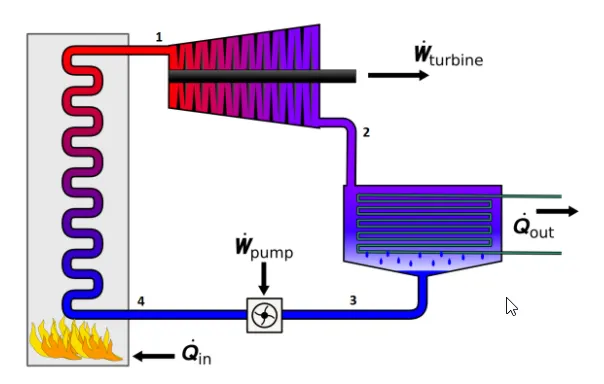
There are four processes in the Rankine cycle. The states are identified by numbers in the T-s diagram.

• Process 1-2: In this process, the working fluid will be pumped from low pressure to high pressure. The fluid is in the liquid form at the start of this process.The water is heated to the saturation temperature, keeping the entropy constant.
• Process 2-3: In case of this process, the high-pressure liquid will enter the boiler. The fluid will be heated at constant pressure with the help of an external heat source andit will become a dry saturated vapor. The required energy needed for heating up can be calculated with the help of an enthalpy entropy chart or steam tables.
• Process 3-4: The dry saturated vapor at the end of the process 2-3 will be expanded through the turbine in this process.It will generate the power. Due to expansion the temperature and the pressure of the vapor will be decreased. Same as the above the output can be easily calculated.
• Process 4-1: At this process, the low temperature and low-pressure vapor will be condensed in the condenser. It will be converted into saturated liquid.

So, these are the four processes in the ideal Rankine cycle.

Incase of the ideal Rankine cycle, the pump and turbine would be isentropic so, they will be generating maximum network output while generating no entropy. Obviously, the actual Rankine cycle will be different from the ideal ones. The losses are accounted and the entropy is varied.

CODE :

% Creating Rankine Cycle Simulator
clear all
close all
clc

disp('      RANKINE CYCLE SIMULATOR      ')

disp('1-2 is Isentropic Expansion in the Turbine')
disp('2-3 is Const Pressure Heat Rejection by the Condenser')
disp('3-4 is Isentropic Compression in the Pump')
disp('4-1 is Const Pressure Heat Addition by the Boiler')
disp(' ')

% Inputs for calculating Rankine cycle
P1 = input('Enter the Pressure at the Turbine Inlet (in bar): ');
T1 = input('Enter the Temperature at the Turbine Inlet (in Degree Celcius): ');
P2 = input('Enter the Pressure at the condensor (in bar): ');
disp('  ')

% Using XSteam function for calculating enthalpy and entropy 
% Enthalpy and Entropy at state 1
H1 = XSteam('h_pT',P1,T1);
S1 = XSteam('s_pT',P1,T1);
hf1 = XSteam('hL_p',P1);
hgl = XSteam('hV_p',P1);
sf1 = XSteam('sL_p',P1);
sg1 = XSteam('sV_p',P1);
T_sat1 = XSteam('Tsat_p',P1);

% State Point 2
S2 = S1;
sf2 = XSteam('sL_p',P2);
sg2 = XSteam('sV_p',P2);

% Dryness Fraction
X2 = (S2 - sf2)/(sg2 - sf2);

hf2 = XSteam('hL_p',P2);
hg2 = XSteam('hV_p',P2);
H2 = hf2 + X2*(hg2 - hf2);
T2 = XSteam('T_ph',P2,H2);
T_sat2 = XSteam('Tsat_p',P2);

% State Point 3
P3 = P2;
T3 = T2;
H3 = hf2;
S3 = sf2;

% State Point 4
P4 = P1;
S4 = S3;
H4 = XSteam('h_ps',P4,S4);
T4 = XSteam('T_ph',P4,H4);

% Calculation of desired quantities
% Work done by Turbine
Wt = H1- H2;

% Work done by Pump
Wp = H4 - H3;

% Net work done
Wnet = Wt - Wp;

% Thermal efficiency
Ntherm = (1 - ((H2 - H3)/(H1 - H4)))*100;

% Back work ratio
BWR = Wp/Wt;

% Specific Steam Conductivity
SSC = 3600/Wt;

% Plotting

% T-S Diagram
t = linspace(0,373.5,200);
figure(1), clf
hold on

% Saturation curve
for i = 1:length(t)
    plot(XSteam('sL_T',t(i)),t(i), 'r.')
    plot(XSteam('sV_T',t(i)),t(i), 'r.')
end

% Rankine Cycle
plot([S1 S2],[T1 T2],'linewidth',2,'Color','k')
text(S1,T1,'1','FontSize',15)

% Beyond saturation curve
if X2>1
    T3 = T_sat2;
    plot([S2 sg2 S3 S4],[T2 T_sat2 T3 T4],'linewidth',2,'color','k')
    T2 = T_sat2;
    text(S2,T2,'2','FontSize',15)
    text(S3,T3,'3','FontSize',15)

    % Beneath saturation curve
else
    plot([S2 S3 S4],[T2 T3 T4],'linewidth',2,'color','k')
    text(S1,T2,'2','FontSize',15)
    text(S3,T3,'3','FontSize',15)
end

n= linspace(T1,T2,500);

for i = 1:length(n)
    plot(XSteam('s_pT',P1,n(i)),n(i),'.','linewidth',2,'color','k')
end

plot([sf1 sg1],[T_sat1 T_sat1], 'linewidth',2, 'color','k')
text(sf1,T_sat1,'4','FontSize',15)

xlabel('Entropy in kJ/kgK')
ylabel('Temperature in K')
title('T-S Diagram')

% H-S Diagram
figure(2), clf
hold on

% Saturation curve
for i = 1:length(t)
    plot(XSteam('sL_T',t(i)),XSteam('hL_T',t(i)), 'r.')
    plot(XSteam('sV_T',t(i)),XSteam('hV_T',t(i)), 'r.')
end

% Rankine Cycle
plot([S1 S2 S3 S4 S1],[H1 H2 H3 H4 H1],'linewidth',2,'color','k')
text(S1,H1,'1','FontSize',15)
text(S2,H2,'2','FontSize',15)
text(S3,H3,'3','FontSize',15)
text(S4,H4+90,'4', 'FontSize',15)

xlabel('Entropy in kJ/kgK')
ylabel('Enthalpy in kJ/kg')
title('H-S Diagram')

% Displaying results in command window
disp('      RESULTS      ')

disp('At state point 1: ')
fprintf('P1 is : %.2f bar \n',P1)
fprintf('T1 is : %.2f Deg Celcius \n',T1)
fprintf('H1 is : %.2f kJ/kg \n',H1)
fprintf('S1 is : %.2f kJ/kgK \n',S1)
disp(' ')

disp('At state point 2: ')
fprintf('P2 is : %.2f bar \n',P2)
fprintf('T2 is : %.2f Deg Celcius \n',T2)
fprintf('H2 is : %.2f kJ/kg \n',H2)
fprintf('S2 is : %.2f kJ/kgK \n',S2)
fprintf('X2 is : %.2f kJ/kgK \n',X2)
disp('  ')

disp('At state point 3: ')
fprintf('P3 is : %.2f bar \n',P3)
fprintf('T3 is : %.2f Deg Celcius \n',T3)
fprintf('H3 is : %.2f kJ/kg \n',H3)
fprintf('S3 is : %.2f kJ/kgK \n',S3)
disp('  ')

disp('At state point 4: ')
fprintf('P4 is : %.2f bar \n',P4)
fprintf('T4 is : %.2f Deg Celcius \n',T4)
fprintf('H4 is : %.2f kJ/kg \n',H4)
fprintf('S4 is : %.2f kJ/kgK \n',S4)
disp('   ')

fprintf('Wt is : %.2f kJ/kg \n', Wt)
fprintf('Wp is : %.2f kJ/kg \n', Wp)
fprintf('Wnet is : %.2f kJ/kg \n', Wnet)
fprintf('Ntherm is : %.2f Percent \n', Ntherm)
fprintf('BWR is : %.2f \n', BWR)
fprintf('SSC is : %.2f kg/kWh \n', SSC)

EXPLANATION :

• Create three prompts to get the inputs from the user and store the corresponding input in the appropriate state point variable. The working fluid is at state point 1 at the inlet of the turbine. Hence store inlet temperature in T1, inet pressure in P1 and exit pressure in P2.
• Using XSteam() function, obtain the enthalpy, entropy and temperature of the saturation vapour. XSteam() takes the name of the data seeked and the corresponding state point values as input arguments. In the first argument, V stands for saturated vapour, L for saturated liquid, h for enthalpy and so on.
• In order to calculate the dryness fraction, first obtain the values of entropy of saturated liquid and vapour at pressure P2 using XSteam() and substitute in the formula. Obtain the values of enthalpy and temperature of saturated vapour at pressure P2. Check for the dryness fraction to calculate the state point 2 values.
• If X2 = 1, then it is saturated vapour. In this case state point 2 properties are equal to properties at saturated vapour line at P2. 1f X2<, then the water is mixture of liquid and vapour. In this case, obtain enthalpy value by supplying pressure P2 and dryness fraction value. T2 will be same as saturation temperature at P2.1f X2>1, the water is still superheated steam. T2 and H2 values are obtained by using Xsteam() for P2 and S2 values.
• At state point 3, pressure at this point remains the same, T3,S3 and H3 values are obtained for saturated liquid at pressure P3.
• At state point 4, entropy remains the same. And pressure increases back to P1 level, as ideal Rankine cycle is reversible. T4 and H4 values are obtained by using function of P4 and S4 values.
• Net work done and back work ratio are calculated by substituting the enthalpy values.
• Then data for the diagram is prepared. Temperature values are created from 0 deg Celcius to critical temperature using linspace(). For all the values of temperature, enthalpy and entropy values are obtained for saturated liquid phase and stored in arrays.
• Using figure command, two different figures are created for T-S and H-S diagram.
• Plot command is used to plot the diagrams for saturated water first and then for rankine cycle. text command is used to mark all the points on the plot.
• Display the steps of the Rankine cycle and result in the command window using disp() and fprintf() commands.

OUTPUT :

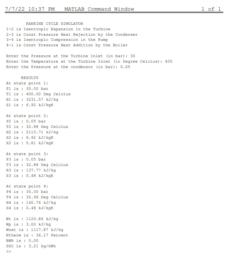
• Net Work Output = 1117.87 kJ/kg
• Back Work Ratio = 0.00267

1. Output Screen -

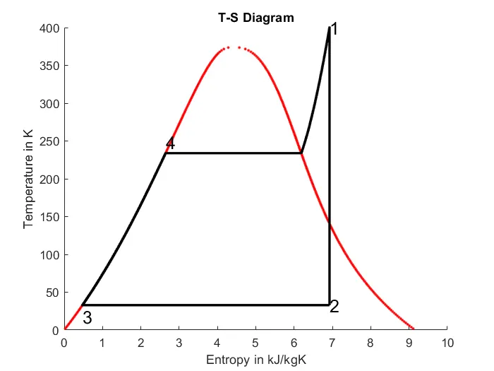
2. T - S Diagram of the Rankine Cycle -

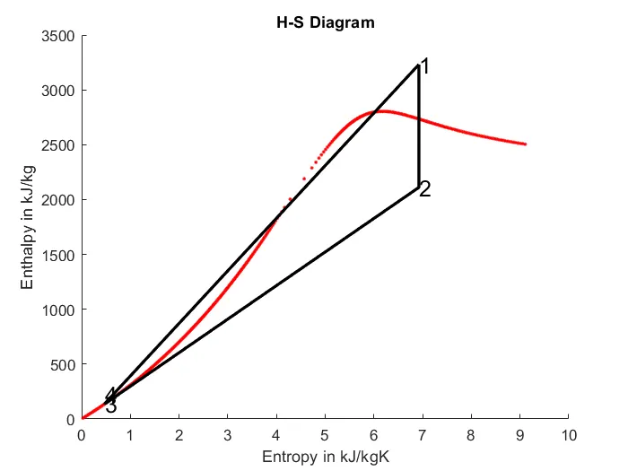
3. H - S Diagram of the Rankine Cycle -

5. CONCLUSION

1. The Rankine Cycle Simulator has been established with required inputs fed and the values of Pressure, Temperature,Enthalphy and Entropy for different state points and also the Work, Efficiency, Back work ratio and specific steam conductivity was calculated.

2. The graph of T-S and H-S for Rankine Cycle was plotted.