Week 3 - Solving second order ODEs

1. AIM :

To simulate the pendulum motion in Matlab.

2. GOVERNING EQUATION :

This ODE represents the equation of motion of a simple pendulum with damping.

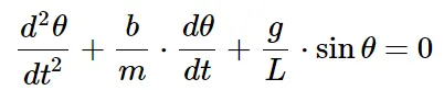
g = gravity in m/s2,

L = length of the pendulum in m,

m = mass of the ball in kg,

b = damping coefficient.

To solve this ODE we need to reduce the order of equation into lower order.

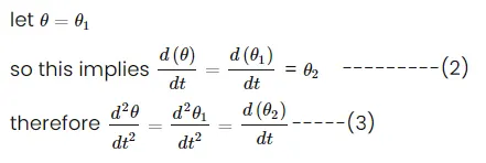
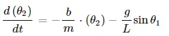
putting these equations, we get

3.OBJECTIVES :

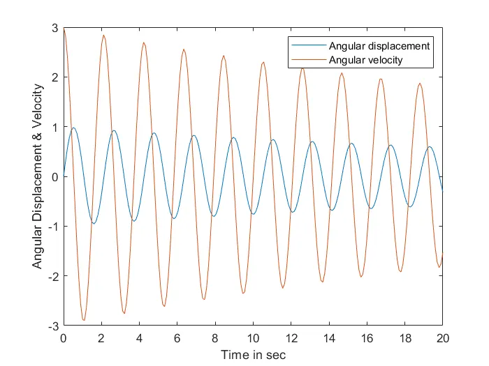
1.Plot displecement and angular velocity with respect to time.

2.Simulate and animate the motion of the pendulum.

4.BODY OF THE CONTENT :

In Engineering, ordinary differential equation (ODE) is used to describe the transient behavior of a system. An ODE is a differential equation containing one or more functions of one independent variable and the derivatives of those functions. The term ordinary is used in contrast with the term partial differential equation which may be with respect to more than one independent variable.

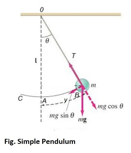
Simple Pendulum - The simple pendulum is an idealized mathematical model of a pendulum.This is a weight (or bob) on the end of a massless cord suspended from a pivot, without friction. When given an initial push, it will swing back and forth at a constant amplitude. Real pendulums are subject to friction and air drag, so the amplitude of their swings declines.

Use,

• Length (L)= 1 m
• Mass (m) = 1 kg
• Dambing cefficient (b) = 0.05
• Gravity (g) = 9.81 m/s2
• Simulate the motion between 0-20 sec
• Angular displacement=0
• Angular velocity=3 rad/sec
• at time t=0.

CODE :

% Solving the second order ODE
clear all
close all
clc

% Input
% Damping coefficient
b = 0.05;

% Length of pendulun in metre
L = 1;

% Mass of the bob in kg
m = 1;

% Gravity in m/s^2
g = 9.81;

% Initial condition zero Angular displacement and angular velocity is 3rad/sec
theta_0 = [0;3];

% time period 0 to 20 sec with 200 values.
t_span = linspace(0,20,200);

% ode 45 function to solve second order ode
[t,results] = ode45(@(t,theta) ode_func(t,theta,b,g,L,m), t_span,theta_0);

% plotting
figure(1)
plot(t,results(:,1))
hold on
plot(t,results(:,2))
xlabel('Time in sec')
ylabel('Angular Displacement & Velocity')
legend('Angular displacement','Angular velocity')

% count command for iterations
ct = 1;

for i = 1 : length(results(:,1))

% fixed coordinates of one end of simple pendulum
x0 = 0;
y0 = 0;

% moving coodinates of the bob
x1 = L*sin(results(i,1));
y1 =-L*cos(results(i,1));

figure(2)
plot([-0.5 0.5],[0 0], 'linewidth',2,'color','g')
hold on
plot([x0 x1],[y0 y1],'LineWidth',1,'Color','b')
plot(x0,y0,'o','markersize',5,'markerfacecolor','r')
plot(x1,y1,'o','MarkerSize',20,'markerfacecolor','r')
% axis setting
axis([-1.5 1.5 -1.5 0.5])
pause(0.01)

M(ct) = getframe(gcf)
ct=ct+1;
hold off

end

% for creating animation video
movie(M)
videofile = VideoWriter('simple_pendulum.avi','Uncompressed AVI');
open(videofile)
writeVideo(videofile,M)
close(videofile)

Code for function 'ode_func' -

function [dtheta_dt] = ode_func(t,theta,b,g,L,m)
theta1 = theta(1);
theta2 = theta(2);

% First ODE
dtheta1_dt = theta2;

% Second ODE
dtheta2_dt = -(b/m)*theta2 - (g/L)*sin(theta1);

dtheta_dt = [dtheta1_dt;dtheta2_dt];

end

Explanation :

• Clear all, close all, clc are used to clear the work space, to clear the graphs that's exists, and clear the command window.
• t_span command used in the ode45 solver which specifies the time span of the iterations that are going to solve the ordinary differential equation.
• ode45 is a function in MATLAB that solves ordinary or partial differential equations using a numerical method. In this problem the highest order is 2. So, we have to take two constant values so that the equation is changed to simple differential equation. The function should take at least 2 inputs to solve the equation to the approximate result.
• plot command is used to plotting the values for the angular velocity and the displacement.
• label commandis used to label the X & Y axis.
• legend command is used to label the angular velocity and the displacement.
• for loop is used to create the specified set of points to keep the bob at different locations, is used to animate the motion of simple pendulum.
• markersize command to create the mass at the end of the pendulum rod.
• axis command is used for fixing axes, x- limits and y-limits.
• pause command is used to slow down the output.
• getframe command is used to get individual frame and stored in variable M.
• movie command is used to create a movie of the individual frame.
• VideoWriter command is used to create a Vídeo file of the movie created and save in the PC.
• close command is used to close the video file.

OUTPUT :

1. Angular displacement and velocity plot with respect to time.

2. Animation of simple pendulum.

5.CONCLUSION :

Establishing a clear view of the transient behavior of the simple pendulum by solving the second order ODE defining its motion. Simulate and animate the motion of the pendulum and Plot the figure of displecement and angular velocity with respect to time.