Week 4.1 - Genetic Algorithm

1. AIM :

To optimise the stalagmite function and find the global maxima of the function.

2. GOVERNING EQUATIONS :

1. Expalin the concept of genetic algorithm and the syntax for ga in MATLAB.

2. To optimise the stalagmite function and find the global maxima of the function.

3. Plot graphs for all 3 studies and for F maximum vs no. of iterations.

3. OBJECTIVES :

Stalagmite Function -

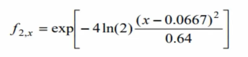
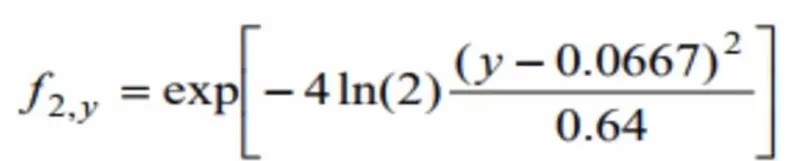
A stalagmite is an upward-growing mound of mineral deposits that have precipitated from water dripping onto the floor of a cave. The figures we get is in the shape of stalagmite so we use this name here. These formulas are represented in the below code.

where,

4. BODY OF THE CONTENT :

GENETIC ALGORITHMS

Genetic Algorithm (GA) are adaptive heuristic search algorithms that belong to the larger part of evolutionary algorithms. Genetic algorithms are based on the ideas of natural selection and genetics. These are intelligent exploitation of random search provided with historical data to direct the search into the region of better performance in solution space. They are commonly used to generate high-quality solutions for optimization problems and search problems.
Genetic algorithms simulate the process of natural selection which means those species who can adapt to changes in their environment are able to survive and reproduce and go to next generation. In simple words, they simulate “survival of the fittest” among individual of consecutive generation for solving a problem. Each generation consist of a population of individuals and each individual represents a point in search space and possible solution. Each individual is represented as a string of character/integer/float/bits. This string is analogous to the Chromosome.

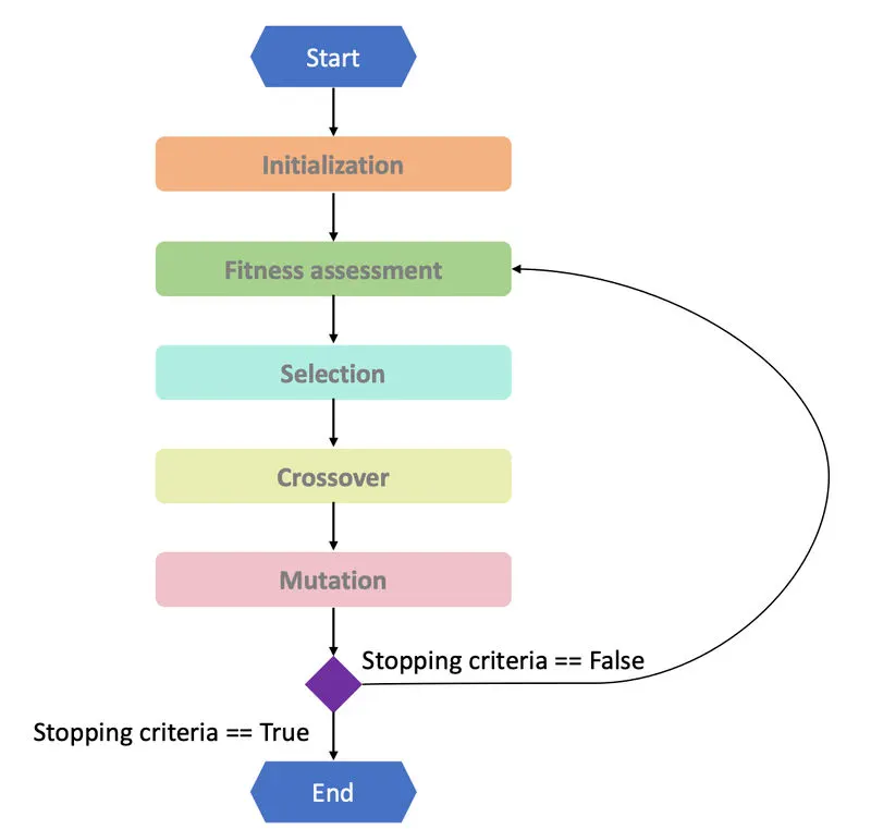
The genetic algorithm starts with a randomly generated population of size M. During the process of iteration, a new population of the same size is generated from the current population using three basic operations on the individuals of the population.

Five phases are considered in a genetic algorithm.

1. Initial population
2. Fitness function
3. Selection
4. Crossover
5. Mutation

GA SYNTAX

The genetic algorithm uses three main types of rules at each step to create the next generation from the current population,

• Selection rules select the individuals, called parents, that contribute to the population at the next generation.
• Crossover rules combine two parents to form children for the next generation.
• Mutation rules apply random changes to individual parents to form children.

1. x = ga(fun,nvars)

Find a local unconstrained minimum, x, to the objective function fun. nvars is dimension of fun.

2. x = ga(fun,nvars,A,b)

Find a local minimum x to fun, subject to the linear inequalities A*x<=b ga evaluates the matrix product A*x as if x is transposed (A*x')

3. x = ga(fun,nvars,A,b,Aeq,beq)

Find a local minimum x to fun, subject to the linear equalities Aeg*x = beq and A*x<=b (Set A=[] and b=[] if no linear inegualities exist). ga evaluates the matrix product Aeq*x as if x is transposed (Aeq*x').

4. x = ga(fun,nvars,A,b Aeq,beq,lb,ub)

Defines a set of lower and upper bounds on the design variables, x, so that a solution is found in the range lb<=x<= ub (Set Aeg=[] and beq=[] if no linear equalities exist).

5. x = ga(fun,nvars,A,b,Aeq,beq,lb,ub,nonlcon)

Subjects the minimization to the constraints defined in nonlcon. The function nonlcon accepts x and returns vectors C and Ceq, representing the nonlinear inegualities and equalities respectively. ga minimizes the fun such that C(x)<=0 and Ceq(x) =0 (Set Ib=[] and ub=[] if no bounds exist).

6. x = ga(fun,nvars,A,b,Aeq,beq,lb,ub,nonlcon,options)

Minimizes with the default optimization parameters replaced by values in options (Set nonlcon=[] if no non linear constraints exist). Create options using optimoptions.

7. x = ga(fun,nvars,A,b,Aeq,beq,lb,ub,nonlcon,IntCon)

Requires that the variables listed in IntCon take integer values.

8. x = ga(problem)

Finds the minimum for problem, where problem is a structure.

9. [x,fval] = ga(_ _)

For any previous input arguments, also returns fval, the value of the fitness function at x.

10. [x,fval,exitflag,output] = ga(_ _)

Also returns exitflag, an integer identifying the reason the algorithm terminated, and output, a structure that contains output from each generation and other information about the performance of the algorithm.

11. [x,fval,exitflag,output,poputation,scores] = ga(_ _)

Also returns a matrix population, whose rows are the final population, and a vector scores, the scores of the final population.

Where,

• Fun - Function
• Nvars - Number of Variables
• A - Linear inequality constraints
• B - Linear inequality constraints
• Aeq - Linear equality constraints
• beq - Linear equality constraínts
• lb - Lower bounds
• ub - Upper bounds
• nonlcon - Non linear constraints
• IntCon - Integer constraints

CODE :

% Optimise the stalagmite function
clear all
close all
clc

% Defining our search space
x = linspace(0,0.6,150);
y = linspace(0,0.6,150);

% Total no. of iterations to run
num_cases = 50;

% Creating a 2D Meshgrid function
[xx yy] = meshgrid(x,y);

% Evaluting the stalagmite function
for i = 1:length(xx)
    for j = 1:length(yy)
        input_vector(1) = xx(i,j);
        input_vector(2) = yy(i,j);
        f(i,j) = stalagmite(input_vector);
    end
end

% Study 1-Statistical behavior
% Study time count start
tic
for i = 1:num_cases
    [inputs, fopt(i)] = ga(@stalagmite,2)
    xopt(i) = inputs(1);
    yopt(i) = inputs(2);
end

% Study time count end
study1_time = toc

% Plotting Unbounded inputs
figure(1)

% To combine two or more plot in one figure
subplot(2,1,1)
hold on

% To contour plot under surface plot
surfc(xx,yy,-f)
xlabel('X values')
ylabel('Y values')

% To set color shading properties
shading interp

plot3(xopt,yopt,-fopt,'marker','o','markersize',3,'markerfacecolor','r');

% Labeling title of figure
title('Unbounded Inputs')
subplot(2,1,2)

% Plot f values
plot(-fopt)
xlabel('Iterations')
ylabel('Function maximum')

% Study 2-Statistical behavior with upper and lower bounds
tic
for i = 1:num_cases
    [inputs,fopt(i)]=ga(@stalagmite,2,[],[],[],[],[0,0],[1;1]);
    xopt(i) = inputs(1);
    yopt(i) = inputs(2);
end
study2_time = toc

figure(2)
subplot(2,1,1)
hold on;

surfc(xx,yy,-f)
xlabel('X values')
ylabel('Y values')
shading interp

plot3(xopt,yopt,-fopt,'marker','o','markersize',3,'markerfacecolor','r');
title('Bounded Inputs')
subplot(2,1,2)

plot(-fopt)
xlabel('Iterations')
ylabel('Function maximum')

% Study 3-Increasing GA iterations
% Create optimization options
options = optimoptions('ga');
options = optimoptions(options,'populationsize',250);
tic
for i = 1:num_cases
    [inputs,fopt(i)]=ga(@stalagmite,2,[],[],[],[],[0,0],[1;1],[],[],options);
    xopt(i) = inputs(1);
    yopt(i) = inputs(2);
end
study3_time = toc

figure(3)
subplot(2,1,1)
hold on

surfc(xx,yy,-f)
xlabel('X values')
ylabel('Y values')
shading interp

plot3(xopt,yopt,-fopt,'marker','o','markersize',3,'markerfacecolor','r');
title('Bounded inputs with modified population size')
subplot(2,1,2)

plot(-fopt)
xlabel('Iterations')
ylabel('Function maximum')

Function code :

If we did not multiply by -1, ga in default calculate the minimum value.

function [f]= stalagmite(input_vector)

f1x = (sin(5.1*pi*input_vector(1)+0.5)).^6;
f1y = (sin(5.1*pi*input_vector(2)+0.5)).^6;
f2x = exp(((-4.*log(2))*(((input_vector(1)-0.0667).^2)/0.64)));
f2y = exp(((-4.*log(2))*(((input_vector(2)-0.0667).^2)/0.64)));
f = -(f1x*f1y*f2x*f2y);

end

EXPLANASION

• Firstly, creating the mesh from the two vectors which will be acting as a search space to find the maxima of the function.
• Creating the mesh of these two vectors using the ‘mesh’ command and defining the no. of iterations as num_cases to iterate the values of the optimum values of the function.
• Now calculating the values of fitness function at each point of the mesh grid formed.
• Now creating its surface through ‘surfc’ command which will also provide the contour of the generated surface.
• While using surfc applying the -ve sign to the function will generate the surface upside down which will be quite good to get the maxima of the function, as it will provide positive value for the maxima using the -ve sign.
• The study behaviour for figure 2 with bounded inputs includes calling our predefined function as in study behaviour 1. The only difference between 1 and 2 is, the plot 2 will have different syntax of ga such that it will define along with the range of inputs.

OUTPUT

study 1

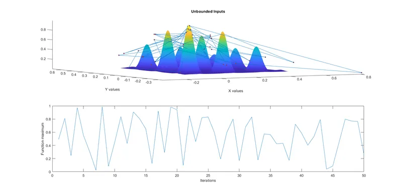
From the above plot we can see that some of our x and y values are out of define boundary conditions (x and y values should be between 0 and 0.6). Some of x and y values are away from salagmite suface. So we failed to reach global maxima in this case. To get global maxima we have to set the bound values.

study 2

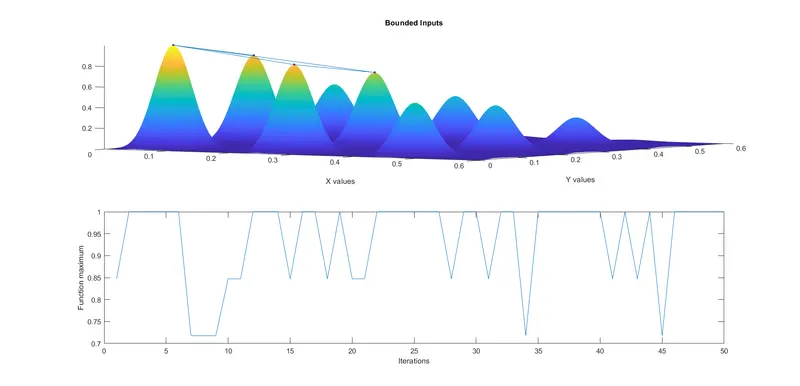
In this study we set upper and lower bound values of x and y in order to get optimum values of x and y. This study gave the better results compare to previous one but not enough to get global maxima. From the plot we are getting four point, which means that our global maxima is lying under the boundary of these four points. So, far more we come up to one concluion that that if we increased the population size than we can get global maxima.

study 3

In study 3, we increased the population size to get the global maxima. In ga, it takes by default population size 50. From the population size of 50 we were unable to get the global maxima so it was necessary to increased to higher value for study. Here, we take population size of 250 and gave the better results compare to previous one. If we give population size 350 we can get global maxima.

5. CONCLUSION :

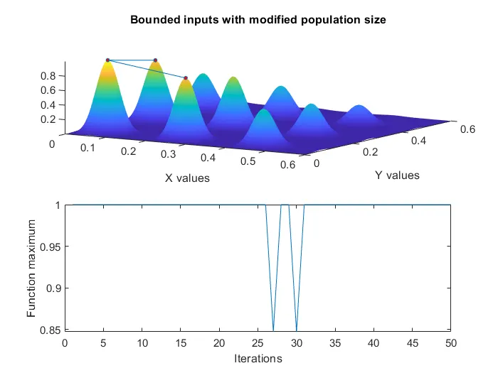
The stalagmite function is optimized and the global maxima for the function is determined. Finding the Global maxima of a function manually is hard and requires time, but we can find how to get the global maxima as well as optimize the stalgmite function easily using MATLAB.