To develop a Rankine Cycle Simulator using MATLAB®
Aim- To develop a Rankine Cycle Simulator using MATLAB®
Objectives-
- Inputs for Turbine Inlet and Outlet will be provided.
- Data entered will be used to find state points in the process.
- Graphs will be plotted between Temperature-Entropy (T-S) & Enthalpy-Entropy (H-S)
- Efficiency and other parameters will be computed based on the user input
- Making an app using MATLAB App Designer
Introduction-
Rankine Cycle: Ideal cycle for Vapour power cycles
The Rankine cycle first developed in the year 1859 by Scottish Engineer William J.M. Rankine is a process in which the chemical energy of the fuel is converted to mechanical energy by superheating the steam in the boiler and then condensing it in the condenser.
It consists of the following four processes-
- Process 1-2 is Isentropic Expansion in Turbine
- Process 2-3 is Constant Pressure Heat Rejection by Condenser
- Process 3-4 is Isentropic Compression in Pump
- Process 4-1 is Constant Pressure heat Addition by Boiler
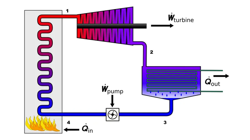
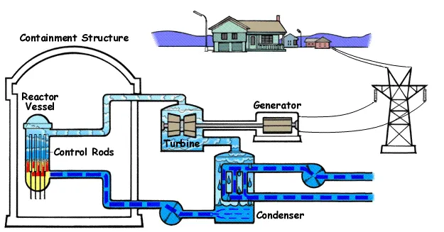
Superheated Steam from the boiler enters the turbine at state 1, where it expands isentropically and produces work by rotating the shaft which is further connected to an electric generator. During expansion, the pressure and temperature of the steam drops to state 2 where steam enters the condenser. Here, the steam is in a saturated liquid-vapour mixture. Steam is condensed at constant pressure in the condenser.
Steam leaves the condenser as saturated liquid and enters the pump and is compressed isentropically to the operating pressure of the boiler. Water enters the boiler as a compressed liquid at state 4 and leaves as superheated steam at state 1.
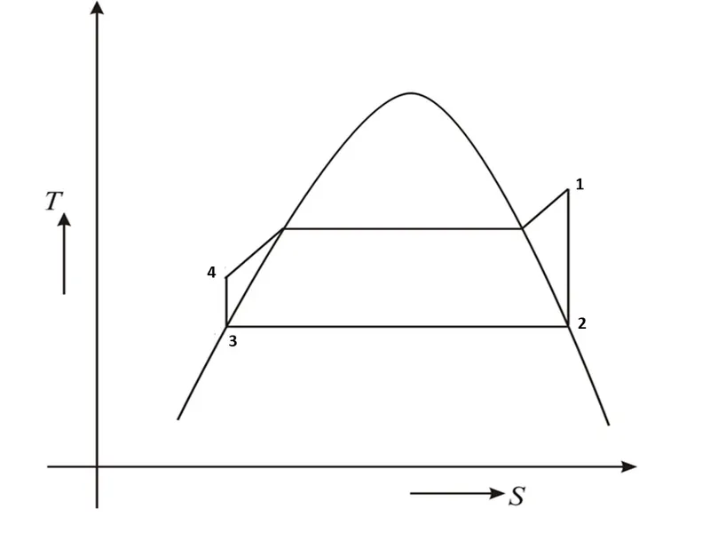
The Rankine cycle can be analysed as a steady flow process. The boiler and condenser do not produce work, also the pump and the turbine are assumed to be isentropic.
Thus,
| Pump (q=0) | `W_p=h_4-h_3` |
| Boiler (w=0) | `q_("in")=h_1-h_4` |
| Turbine (q=0) | `W_t=h_1-h_2` |
| Condenser (w=0) | `q_(out)=h_2-h_3` |
| Net Work | `W=W_t-W_p` |
| Thermal Efficiency | `η_(th)=w/q_("in")` |
| Back Work Ratio | `BW_(ratio)=W_p/W_t` |
Increasing the efficiency of Rankine Cycle -
Ideal Reheat Rankine Cycle-
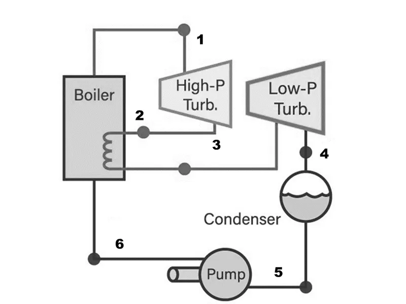
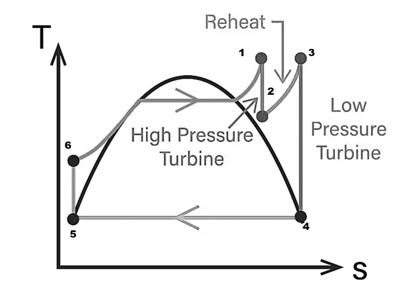
Reheating is done to improve the efficiency of the Rankine cycle. Here the expansion takes place in two stages i.e. first the steam is expanded isentropically by a high pressure turbine to an intermediate pressure and then sent back to the boiler where it gets reheated at constant pressure and then steam is sent to expand in the second stage by a low pressure turbine to the condenser pressure.
Thus, the net-work output and heat input for the reheat case becomes
`W=(h_1-h_2+h_3-h_4 )-(h_6-h_5 )`
`q_"in"=(h_1-h_6+h_3-h_2 )`
Ideal Regenerative Rankine Cycle-
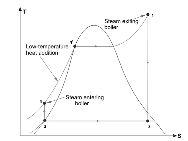
From the T-S diagram it is clear that state (4-4’) a lot of heating goes on to bring the liquid up to the boiling point at that pressure at a relatively low temperature, thus reducing heat-addition temperature and the cycle efficiency.
To overcome this & to increase efficiency regeneration is used where we try to increase the temperature of the liquid leaving the pump before entering the boiler. This is achieved by bleeding or extracting steam from the turbine at various points to heat the feedwater (water to be supplied to a boiler for conversion into steam) inside a feedwater heater.
Feedwater inside the heater can be heated in two ways-
Open Feedwater Heater- here the steam extracted from the turbine mixes with the feedwater exiting the pump, the mixture leaves the heater as a saturated liquid at the heater pressure.
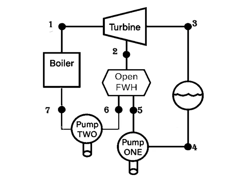
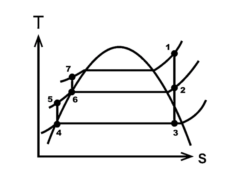
In the Rankine Regenerative cycle steam enters the turbine at (1) and expands isentropically in the turbine till the point (2) where it is extracted. At state (2) some amount of heat is taken and fed to the feedwater heater while the rest steam continues to expand in the turbine till it reaches the condenser pressure at point (3). From the condenser the steam leaves as saturated liquid at condenser pressure (4). The feedwater enters into the open feedwater heater via pump (1) where it mixes with the steam extracted from turbine at (2). The mixture leaves the heater as saturated liquid at heater pressure (6). Pump (2) raises the feedwater heater pressure to boiler pressure (7), inside the boiler phase change from water to steam occurs and then superheating of steam takes place.
If boiler generates 1 kg of steam and m kg of steam is extracted at (2) so (1-m) kg steam expands completely.
`q_"in"=h_1-h_7`
`q_(out)=1-m(h_3-h_3 )`
`W_t=h_1-h_2+1-m(h_2-h_3 )`
`W_p=1-m(h_5-h_4 ) +h_7-h_6`
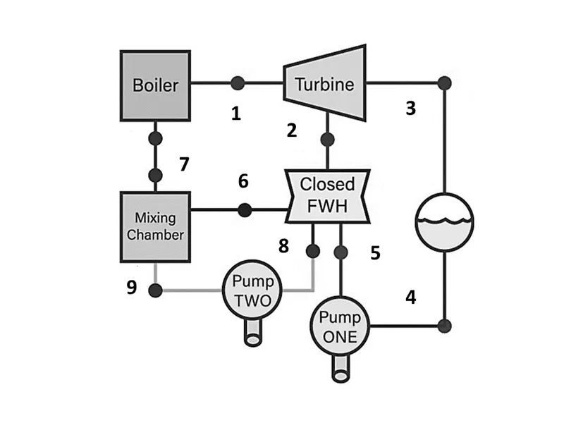
Closed Feedwater Heater-here heat is transferred from the extracted steam to the feedwater without mixing
MATLAB Implementation-
To make the simulator, MATLAB App Designer was used along with MATLAB scripts in this project. All the scripts, functions and apps of this project are available on my GitHub link for the latter is given below-
GitHub Repository Link...
Code Explanation-
https://github.com/mastersinusoidal/Rankine-Cycle-Simulator/blob/main/rankine_cycle_simulator.m
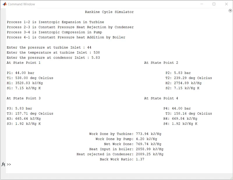
- First, Input parameters were asked from user to parameterise the simulator.
clear all                               % Clears command history
close all                               % Closes  all windows
clc                                     % Clears command window

% Basic Info
fprintf('%60s rn', 'Rankine Cycle Simulator')
fprintf('%s n','Process 1-2 is Isentropic Expansion in Turbine')
fprintf('%s n','Process 2-3 is Constant Pressure Heat Rejection by Condenser')
fprintf('%s n','Process 3-4 is Isentropic Compression in Pump')
fprintf('%s rn','Process 4-1 is Constant Pressure heat Addition by Boiler')

%% INPUTS
p1=input('Enter the pressure at turbine Inlet : ');
t1=input('Enter the temperature at turbine Inlet : ');
p2=input('Enter the pressure at condensor Inlet : ');
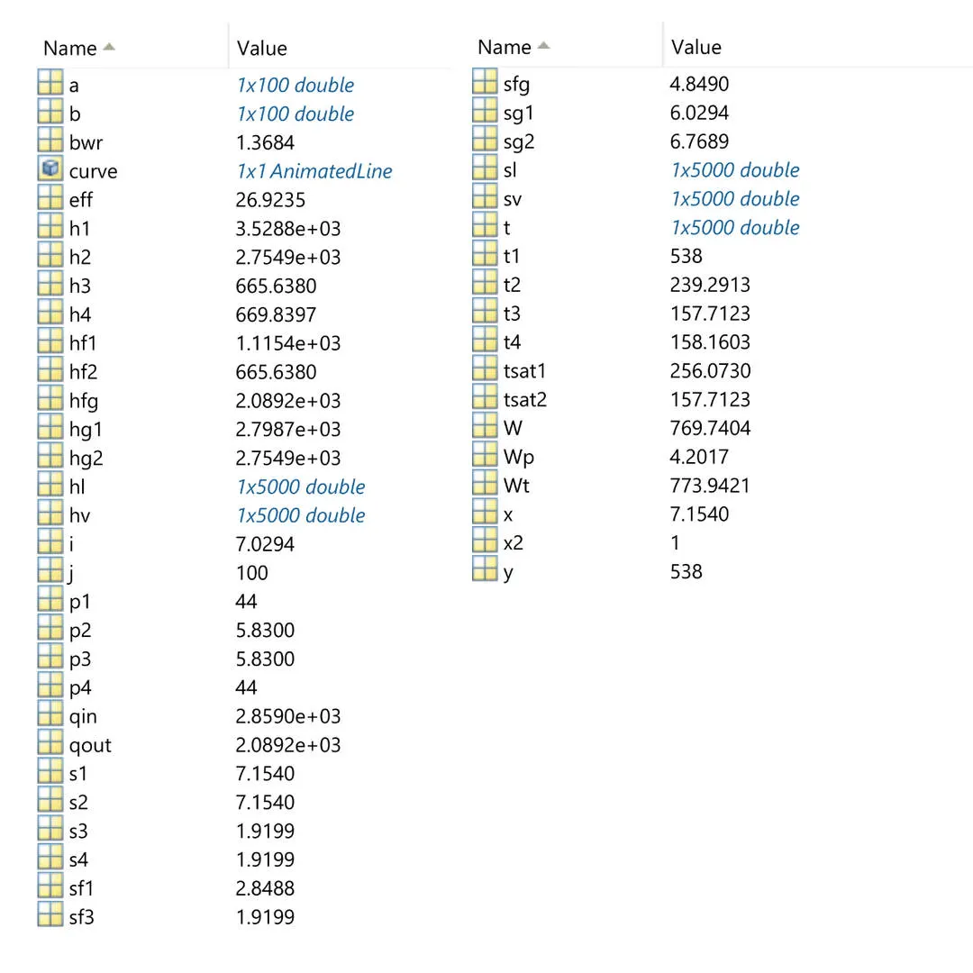
- State points properties (Pressure, Temperature, Entropy, Enthapy) are calculated based on the values from the XSteam.m file.
%% 1-2 Isentropic Turbine Expansion
h1=XSteam('h_pT',p1,t1);
s1=XSteam('s_pT',p1,t1);
tsat1=XSteam('Tsat_p',p1);     %Saturation Temp.at p1
hg1=XSteam('hV_p',p1);
hf1=XSteam('hL_p',p1);
sg1=XSteam('sV_p',p1);
sf1=XSteam('sL_p',p1);

s2=s1;
hf2=XSteam('hL_p',p2);
sf3=XSteam('sL_p',p2);
hg2=XSteam('hV_p',p2);
sg2=XSteam('sV_p',p2);
sfg=sg2-sf3;                    %entropy of wet region
hfg= hg2-hf2;
if s2 < sg2                     % Checks to see if Point 2 is within the vapor dome
     x2=(s2-sf3)/sfg;           % calculates the new quality at this point
     h2=hf2+x2*hfg;             % calculates the new enthalpy
else
     x2 = 1;                    % Quality is max 1
     h2 = x2*hg2;               % calculates the new enthalpy
end
t2=XSteam('T_ps',p2,s2);
tsat2=XSteam('Tsat_p',p2);      %Saturation Temp.at p2
%% 2-3 Isobaric Condenser
p3=p2;
s3=sf3;
h3=hf2;
%% 3-4 Isentropic Pump
s4=s3;
t3=tsat2;
%% 4-1 Isobaric Boiler
p4=p1;
h4=XSteam('h_ps',p4,s4);
t4=XSteam('T_ps',p4,s4);- Property Diagrams (T-S & H-S) are animated and drawn next using animatedline and plot functions.
%% T-S & H-S Diagrams
t= linspace(1,t1,5000);

figure(1)
hold on
sl=zeros;
sv=zeros;
hl=zeros;
hv=zeros;
for i=1:length(t)
    sl(i)=XSteam('sL_T',t(i));
    sv(i)=XSteam('sV_T',t(i));
    hl(i)=XSteam('hL_T',t(i));
    hv(i)=XSteam('hV_T',t(i));

end
plot(sl,t,'--r','linewidth',1)
plot(sv,t,'--r','linewidth',1)
%% T-S Diagram Animation
for i=s1:s2
    a=linspace(s1,s2,100);
    b=linspace(t1,t2,100);
    curve=animatedline('color','c','linewidth',2);
    for j=1:100
        x=a(j);
        y=b(j);
        addpoints(curve,x,y);
        pause(0.01) ;
    end
end
for i=sg2:s2
    a=linspace(s2,sg2,100);
    b=linspace(t2,tsat2,100);
    curve=animatedline('color','c','linewidth',2);
    for j=1:100
        x=a(j);
        y=b(j);
        addpoints(curve,x,y);
        pause(0.01) ;
    end
end
for i=s3:sg2
    a=linspace(sg2,s3,100);
    b=linspace(tsat2,t3,100);
    curve=animatedline('color','c','linewidth',2);
    for j=1:100
        x=a(j);
        y=b(j);
        addpoints(curve,x,y);
        pause(0.01) ;
    end
end
for i=s3:s4
    a=linspace(s3,s4,100);
    b=linspace(t3,t4,100);
    curve=animatedline('color','c','linewidth',2);
    for j=1:100
        x=a(j);
        y=b(j);
        addpoints(curve,x,y);
        pause(0.01) ;
    end
end
for i=s4:sf1
    a=linspace(s4,sf1,100);
    b=linspace(t4,tsat1,100);
    curve=animatedline('color','c','linewidth',2);
    for j=1:100
        x=a(j);
        y=b(j);
        addpoints(curve,x,y);
        pause(0.01) ;
    end
end
for i=sf1:sg1
    a=linspace(sf1,sg1,100);
    b=linspace(tsat1,tsat1,100);
    curve=animatedline('color','c','linewidth',2);
    for j=1:100
        x=a(j);
        y=b(j);
        addpoints(curve,x,y);
        pause(0.01) ;
    end
end
for i=sg1:s1
    a=linspace(sg1,s1,100);
    b=linspace(tsat1,t1,100);
    curve=animatedline('color','c','linewidth',2);
    for j=1:100
        x=a(j);
        y=b(j);
        addpoints(curve,x,y);
        pause(0.01) ;
    end
end
%
%plot([s1 s2],[t1 t2],'linewidth',2)
%plot([s2 sg2],[t2 tsat2],'linewidth',2)
%plot([sg2 s3],[tsat2 t3],'linewidth',2)
%plot([s3 s4],[t3 t4],'linewidth',2)
%plot([s4 sf1],[t4 tsat1],'linewidth',2)
%plot([sf1 sg1],[tsat1 tsat1],'linewidth',2)
%plot([sg1 s1],[tsat1 t1],'linewidth',2)

xlabel({'Specific Entropy [S] ','(kJ/kg K)'},'FontWeight','bold')
ylabel({'Temperature [T] ','(Deg C)'},'FontWeight','bold')

%% H-S Diagram Animation
figure(2)
hold on
plot([s1 s2],[h1 h2],'linewidth',2)
plot([s2 s3],[h2 h3],'linewidth',2)
plot([s3 s4],[h3 h4],'linewidth',2)
plot([s4 sf1],[h4 hf1],'linewidth',2)
plot([sf1 sg1],[hf1 hg1],'linewidth',2)
plot([sg1 s1],[hg1 h1],'linewidth',2)
plot([sl sv],[hl hv],'--r','linewidth',1)

xlabel({'Specific Entropy [S] ','(kJ/kg K)'},'FontWeight','bold')
ylabel({'Specific Enthalpy [H] ' ,'(kJ/kg)'},'FontWeight','bold')
- Now, the work and efficiency of the are calculated using the mathematical relations.
%% Efficiency and Work

Wt=h1-h2;
Wp=h4-h3;
W=Wt-Wp;

qin=h1-h4;
qout=h2-h3;

eff=W*100/qin;
bwr=qin/qout;- Finally the output and all the calculated values are displayed on the command window.
%% Display
fprintf('%-60s %20s rn', 'At State Point 1','At State Point 2' )
fprintf('%s %.2f %s %64s %.2f %s n','P1:',p1,'bar','P2:',p2,'bar')
fprintf('%s %.2f %s %55s %.2f %s n','T1:',t1,'deg Celcius','T2:',t2,'deg Celcius')
fprintf('%s %.2f %s %60s %.2f %s n','H1:',h1,'kJ/Kg','H2:',h2,'kJ/Kg')
fprintf('%s %.2f %s %61s %.2f %s rn','S1:',s1,'kJ/Kg K','S2:',s2,'kJ/Kg K')
fprintf('%-60s %20s rn', 'At State Point 3','At State Point 4' )
fprintf('%s %.2f %s %64s %.2f %s n','P3:',p3,'bar','P4:',p4,'bar')
fprintf('%s %.2f %s %55s %.2f %s n','T3:',t3,'deg Celcius','T3:',t4,'deg Celcius')
fprintf('%s %.2f %s %60s %.2f %s n','H3:',h3,'kJ/Kg','H4:',h4,'kJ/Kg')
fprintf('%s %.2f %s %60s %.2f %s rn','S3:',s3,'kJ/Kg K','S4:',s4,'kJ/Kg K')
fprintf('%60s %.2f %s n','Work Done by Turbine:',Wt,'kJ/Kg')
fprintf('%60s %.2f %s n','Work Done by Pump:',Wp,'kJ/Kg')
fprintf('%60s %.2f %s n','Net Work Done:',W,'kJ/Kg')
fprintf('%60s %.2f %s n','Heat Input in boiler:',qin,'kJ/Kg')
fprintf('%60s %.2f %s n','Heat rejected in Condenser:',qout,'kJ/Kg')
fprintf('%60s %.2f n','Back Work Ratio:',bwr)
Function rankine_cycle_reheat.m-
https://github.com/mastersinusoidal/Rankine-Cycle-Simulator/blob/main/rankine_cycle_reheat.m
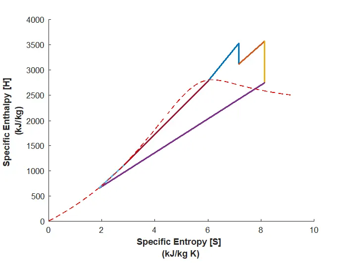
- For Reheat Rankine cycle a function rankine_cycle_reheat was created. This function takes pressure at turbine inlet, temperature at turbine inlet, pressure at condenser inlet and pressure at reheat as inputs. And this also follows the same methedology like the above simple rankine cycle code, first it finds the state point properties then plots the points and calculates the thermal efficiency & work.
function [eff]=rankine_cycle_reheat(t1,p1,p2,p3)
t= linspace(1,t1,5000);

figure(1)
hold on
sl=zeros;
sv=zeros;
hl=zeros;
hv=zeros;
for i=1:length(t)
    sl(i)=XSteam('sL_T',t(i));
    sv(i)=XSteam('sV_T',t(i));
    hl(i)=XSteam('hL_T',t(i));
    hv(i)=XSteam('hV_T',t(i));

end
plot(sl,t,'--r','linewidth',1)
plot(sv,t,'--r','linewidth',1)

h1 = XSteam('h_pT',p1,t1);
s1 = XSteam('s_pT',p1,t1);

s2=s1;
h2=XSteam('h_pS',p2,s2);
t2=XSteam('T_hs',h2,s2);

h3=XSteam('h_pT',p3,t1);
s3=XSteam('s_pT',p3,t1);
t3=t1;

s4=s3;
hf4=XSteam('hL_p',p3);
sf4=XSteam('sL_p',p3);
hg4=XSteam('hV_p',p3);
sg4=XSteam('sV_p',p3);
sfg=sg4-sf4;
hfg= hg4-hf4;
if s4
Function rankine_cycle_regeneration.m-
https://github.com/mastersinusoidal/Rankine-Cycle-Simulator/blob/main/rankine_cycle_regeneration.m
- Similarly the regenerative rankine cycle is also implemented in the same way.
function [eff]=rankine_cycle_regeneration(t1,p1,p2,p3)
t= linspace(1,t1,5000);

figure(1)
hold on
sl=zeros;
sv=zeros;
hl=zeros;
hv=zeros;
for i=1:length(t)
    sl(i)=XSteam('sL_T',t(i));
    sv(i)=XSteam('sV_T',t(i));
    hl(i)=XSteam('hL_T',t(i));
    hv(i)=XSteam('hV_T',t(i));

end
plot(sl,t,'--r','linewidth',1)
plot(sv,t,'--r','linewidth',1)

h1 = XSteam('h_pT',p1,t1);
s1 = XSteam('s_pT',p1,t1);


s2=s1;
h2=XSteam('h_pS',p2,s2);
t2=XSteam('T_hs',h2,s2);

tsat3=XSteam('Tsat_p',p3);

hf3=XSteam('hL_p',p3);
sf3=XSteam('sL_p',p3);
hg3=XSteam('hV_p',p3);
sg3=XSteam('sV_p',p3);
sfg=sg3-sf3;                    %entropy of wet region
hfg= hg3-hf3;
if s2 < sg3                     % Checks to see if Point 2 is within the vapor dome
     x2=(s2-sf3)/sfg;           % calculates the new quality at this point
     h3=hf3+x2*hfg;             % calculates the new enthalpy
else
     x2 = 1;                    % Quality is max 1
     h3 = x2*hg3;               % calculates the new enthalpy
end

s3=s2;


s4=XSteam('sL_p',p3);
hf4=XSteam('hL_p',p3);
sf4=XSteam('sL_p',p3);
hg4=XSteam('hV_p',p3);
sg4=XSteam('sV_p',p3);
sfg=sg4-sf4;

h4= hf4;

tsat4=XSteam('Tsat_p',p3);
t4=XSteam('T_hs',h4,s4);

v4=XSteam('vL_p',p3);
p4=p3;
p5=p2;
h5=h4+v4*((p5-p4)*100);


s5=s4;
t5=t4;


s6=XSteam('sL_p',p2);
s7=s6;

p6=p1;
t6=XSteam('T_ps',p6,s6);
h6=XSteam('h_pS',p6,s6);
sg1=XSteam('sV_p',p1);
hg1=XSteam('hV_p',p1);
sf1=XSteam('sL_p',p1);
hf1=XSteam('hL_p',p1);
tsat1=XSteam('Tsat_p',p1);


tsat2=XSteam('Tsat_p',p2);
t6=tsat2;
sg2=XSteam('sV_p',p2);
hg2=XSteam('hV_p',p2);
sf2=XSteam('sL_p',p2);
hf2=XSteam('hL_p',p2);

t7=XSteam('T_ps',p1,sf2);
t5=XSteam('T_ps',p3,s5);


v7=XSteam('vL_p',p1);
h7=h6+v7*((p1-p2)*100);


m=(h6-h5)/(h2-h5);

hold on

plot([s1 s2],[t1 t2],'linewidth',2)
plot([s2 sg2],[t2 tsat2],'linewidth',2)
plot([sg2 sf2],[tsat2 tsat2],'linewidth',2)
plot([sf2 sf2],[t6 t7],'linewidth',2)
plot([s2 s3],[t2 tsat3],'linewidth',2)
plot([s3 s4],[tsat3 tsat3],'linewidth',2)
plot([s4 s5],[tsat3 t5],'linewidth',2)
plot([s5 s6],[t5 tsat2],'linewidth',2)
plot([s6 s7],[t6 t7],'linewidth',2)
plot([s7 sf1],[t7 tsat1],'linewidth',2)
plot([sf1 sg1],[tsat1 tsat1],'linewidth',2)
plot([sg1 s1],[tsat1 t1],'linewidth',2)
xlabel({'Specific Entropy [S] ','(kJ/kg K)'},'FontWeight','bold')
ylabel({'Temperature [T] ','(Deg C)'},'FontWeight','bold')

figure(2)
hold on

plot([s1 s2],[h1 h2],'linewidth',2)
plot([s2 sg2],[h2 hg2],'linewidth',2)
plot([sg2 sf2],[hg2 hf2],'linewidth',2)
plot([sf2 sf2],[h6 h7],'linewidth',2)
plot([s2 s3],[h2 h3],'linewidth',2)
plot([s3 s4],[h3 h4],'linewidth',2)
plot([s4 s5],[h4 h5],'linewidth',2)
plot([s5 s6],[h5 h6],'linewidth',2)
plot([s6 s7],[h6 h7],'linewidth',2)
plot([s7 sf1],[h7 hf1],'linewidth',2)
plot([sf1 sg1],[hf1 hg1],'linewidth',2)
plot([sg1 s1],[hg1 h1],'linewidth',2)
plot([sl sv],[hl hv],'--r','linewidth',1)
xlabel({'Specific Entropy [S] ','(kJ/kg K)'},'FontWeight','bold')
ylabel({'Specific Enthalpy [H] ' ,'(kJ/kg)'},'FontWeight','bold')


Wp = (1-m)*(h5-h4)+(h7-h6);
Wt = (h1-h2)+(1-m)*(h2-h3);
qin = h1-h7;
qout=(1-m)*h3-h4;
W=Wt-Wp;
eff = (W/qin);
bwr=Wp/Wt;


end
Output-
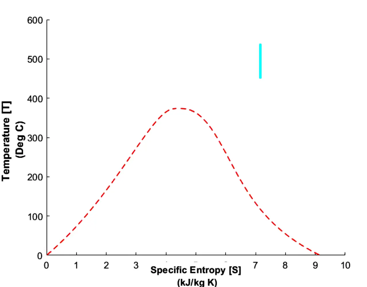
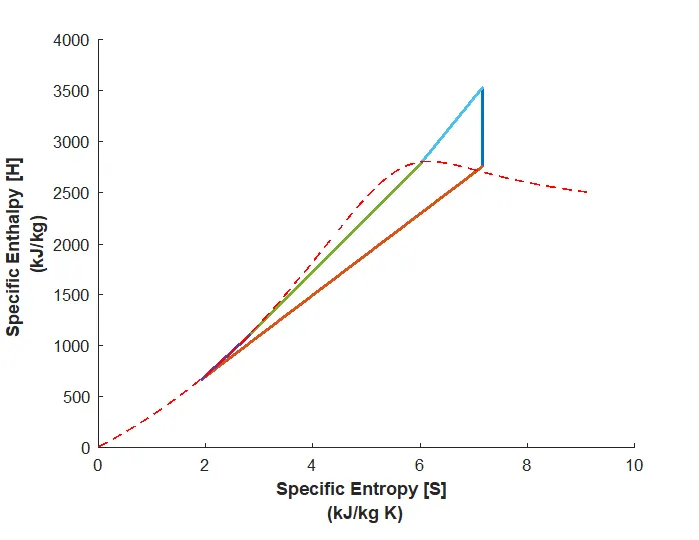
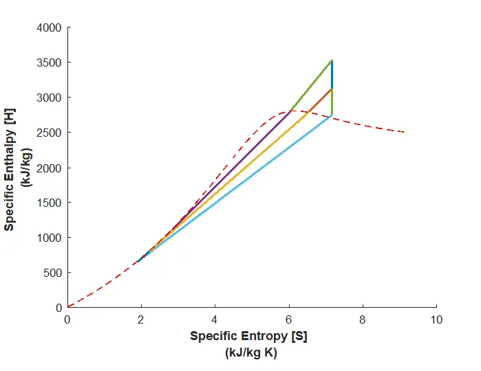
Type the following command to execute reheat rankine cycle.
rankine_cycle_reheat(538,44,12,5.58) 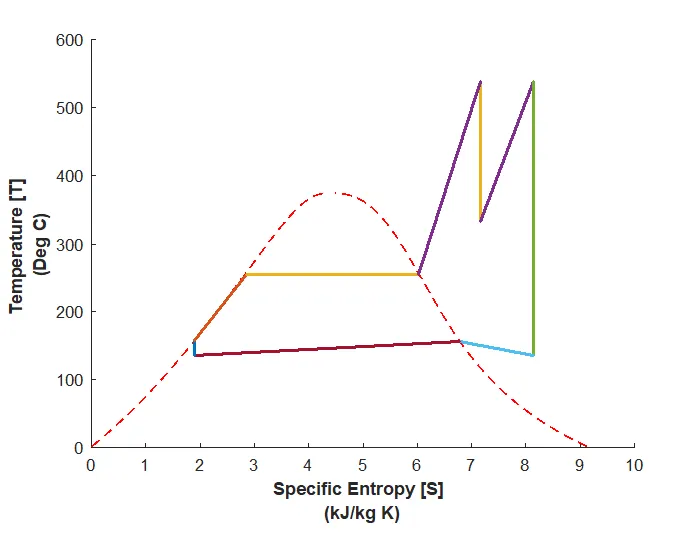
Type the command to execute the regenerative rankine cycle.
rankine_cycle_regeneration(538,44,12,5.58) 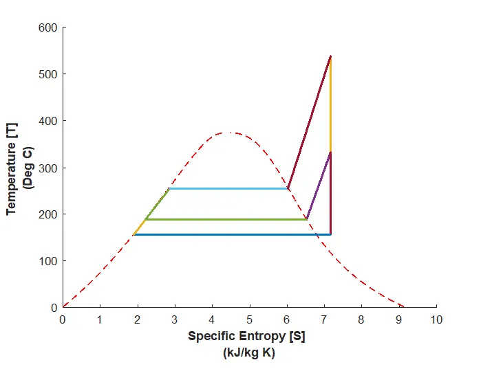
Rankine Cycle Simulator App using MATLAB App Designer-
https://github.com/mastersinusoidal/Rankine-Cycle-Simulator/blob/main/rankine_app.mlapp
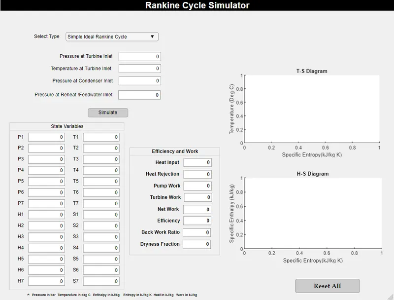
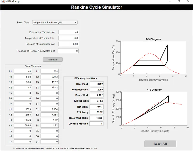
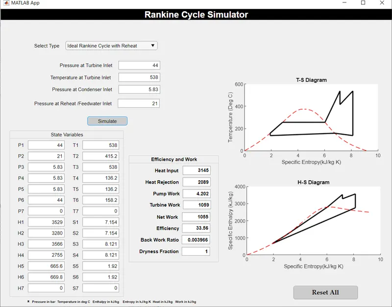
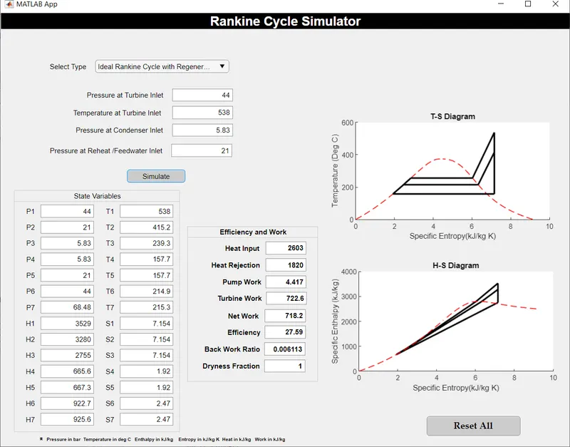
This Simulator simulates three Rankine cycles viz. Simple, Reheat, Regeneration that the user can select from the drop down menu.
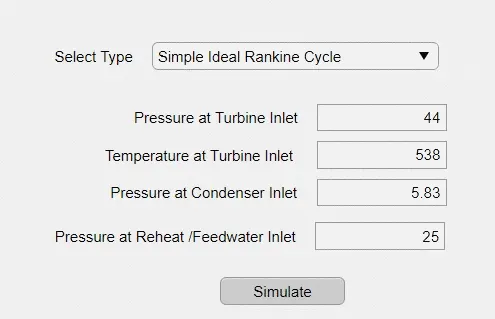
After Selecting the Cycle type next the user needs to input some data in order to parameterise the simulator, then click on Simulate button.
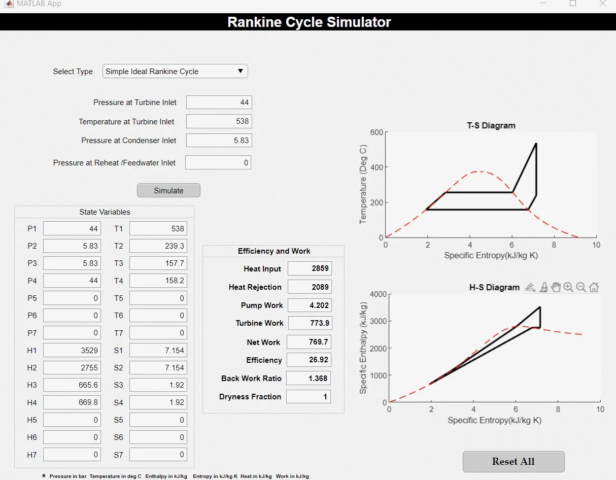
The Reset All button resets the app to let the user simulate for other parameters. This reset like behaviour is achieved by closing the app and opening a new instance for this a callback function was created that hides the currently running instance , opens a second instance with default values, and then deletes the first one.
        function ResetAllButtonPushed(app, event)
            app.UIFigure.Visible='off';
            rankine_app();
            close(app.UIFigure)
        end
Output-
App Code-
https://github.com/mastersinusoidal/Rankine-Cycle-Simulator/blob/main/rankine_app_exported.m
classdef rankine_app_exported < matlab.apps.AppBase
% Properties that correspond to app components
properties (Access = public)
UIFigure matlab.ui.Figure
RankineCycleSimulatorLabel matlab.ui.control.Label
PressureatTurbineInletEditFieldLabel matlab.ui.control.Label
PressureatTurbineInletEditField matlab.ui.control.NumericEditField
TemperatureatTurbineInletEditFieldLabel matlab.ui.control.Label
TemperatureatTurbineInletEditField matlab.ui.control.NumericEditField
PressureatCondenserInletEditFieldLabel matlab.ui.control.Label
PressureatCondenserInletEditField matlab.ui.control.NumericEditField
StateVariablesPanel matlab.ui.container.Panel
GridLayout matlab.ui.container.GridLayout
P1EditFieldLabel matlab.ui.control.Label
P1 matlab.ui.control.NumericEditField
P2EditFieldLabel matlab.ui.control.Label
P2 matlab.ui.control.NumericEditField
P3EditFieldLabel matlab.ui.control.Label
P3 matlab.ui.control.NumericEditField
P4EditFieldLabel matlab.ui.control.Label
P4 matlab.ui.control.NumericEditField
P5EditFieldLabel matlab.ui.control.Label
P5 matlab.ui.control.NumericEditField
P6EditFieldLabel matlab.ui.control.Label
P6 matlab.ui.control.NumericEditField
P7EditFieldLabel matlab.ui.control.Label
P7 matlab.ui.control.NumericEditField
T1Label matlab.ui.control.Label
T1 matlab.ui.control.NumericEditField
T2Label matlab.ui.control.Label
T2 matlab.ui.control.NumericEditField
T3Label matlab.ui.control.Label
T3 matlab.ui.control.NumericEditField
T4Label matlab.ui.control.Label
T4 matlab.ui.control.NumericEditField
T5Label matlab.ui.control.Label
T5 matlab.ui.control.NumericEditField
T6Label matlab.ui.control.Label
T6 matlab.ui.control.NumericEditField
T7Label matlab.ui.control.Label
T7 matlab.ui.control.NumericEditField
H1EditFieldLabel matlab.ui.control.Label
H1 matlab.ui.control.NumericEditField
H2EditFieldLabel matlab.ui.control.Label
H2 matlab.ui.control.NumericEditField
H3EditFieldLabel matlab.ui.control.Label
H3 matlab.ui.control.NumericEditField
H4EditFieldLabel matlab.ui.control.Label
H4 matlab.ui.control.NumericEditField
H5EditFieldLabel matlab.ui.control.Label
H5 matlab.ui.control.NumericEditField
H6EditFieldLabel matlab.ui.control.Label
H6 matlab.ui.control.NumericEditField
H7EditFieldLabel matlab.ui.control.Label
H7 matlab.ui.control.NumericEditField
S1EditFieldLabel matlab.ui.control.Label
S1 matlab.ui.control.NumericEditField
S2EditFieldLabel matlab.ui.control.Label
S2 matlab.ui.control.NumericEditField
S3EditFieldLabel matlab.ui.control.Label
S3 matlab.ui.control.NumericEditField
S4EditFieldLabel matlab.ui.control.Label
S4 matlab.ui.control.NumericEditField
S5EditFieldLabel matlab.ui.control.Label
S5 matlab.ui.control.NumericEditField
S6EditFieldLabel matlab.ui.control.Label
S6 matlab.ui.control.NumericEditField
S7EditFieldLabel matlab.ui.control.Label
S7 matlab.ui.control.NumericEditField
UIAxes matlab.ui.control.UIAxes
UIAxes_2 matlab.ui.control.UIAxes
SimulateButton matlab.ui.control.Button
EfficiencyandWorkPanel matlab.ui.container.Panel
HeatInputEditFieldLabel matlab.ui.control.Label
HeatInputEditField matlab.ui.control.NumericEditField
HeatRejectionEditFieldLabel matlab.ui.control.Label
HeatRejectionEditField matlab.ui.control.NumericEditField
PumpWorkEditFieldLabel matlab.ui.control.Label
PumpWorkEditField matlab.ui.control.NumericEditField
TurbineWorkEditFieldLabel matlab.ui.control.Label
TurbineWorkEditField matlab.ui.control.NumericEditField
NetWorkEditFieldLabel matlab.ui.control.Label
NetWorkEditField matlab.ui.control.NumericEditField
EfficiencyEditFieldLabel matlab.ui.control.Label
EfficiencyEditField matlab.ui.control.NumericEditField
BackWorkRatioEditFieldLabel matlab.ui.control.Label
BackWorkRatioEditField matlab.ui.control.NumericEditField
DrynessFractionEditFieldLabel matlab.ui.control.Label
DrynessFractionEditField matlab.ui.control.NumericEditField
PressureinbarLabel matlab.ui.control.Label
TemperatureindegCLabel matlab.ui.control.Label
EnthalpyinkJkgLabel matlab.ui.control.Label
EntropyinkJkgKLabel matlab.ui.control.Label
HeatinkJkgLabel matlab.ui.control.Label
WorkinkJkgLabel matlab.ui.control.Label
Label matlab.ui.control.Label
SelectTypeDropDownLabel matlab.ui.control.Label
rankinedropdown matlab.ui.control.DropDown
PressureatReheatFeedwaterInletEditFieldLabel matlab.ui.control.Label
PressureatReheatFeedwaterInletEditField matlab.ui.control.NumericEditField
ResetAllButton matlab.ui.control.Button
end
methods (Access = private)
end
methods (Access = public)
end
% Callbacks that handle component events
methods (Access = private)
% Button pushed function: SimulateButton
function SimulateButtonPushed(app, event)
if strcmp(app.rankinedropdown.Value,'Simple Ideal Rankine Cycle')
p1=app.PressureatTurbineInletEditField.Value;
t1=app.TemperatureatTurbineInletEditField.Value;
p2=app.PressureatCondenserInletEditField.Value;
h1=XSteam('h_pT',p1,t1);
s1=XSteam('s_pT',p1,t1);
tsat1=XSteam('Tsat_p',p1);
hg1=XSteam('hV_p',p1);
hf1=XSteam('hL_p',p1);
sg1=XSteam('sV_p',p1);
sf1=XSteam('sL_p',p1);
s2=s1;
hf2=XSteam('hL_p',p2);
sf3=XSteam('sL_p',p2);
hg2=XSteam('hV_p',p2);
sg2=XSteam('sV_p',p2);
sfg=sg2-sf3;
hfg= hg2-hf2;
if s2 < sg2
x2=(s2-sf3)/sfg;
h2=hf2+x2*hfg;
else
x2 = 1;
h2 = x2*hg2;
end
t2=XSteam('T_ps',p2,s2);
tsat2=XSteam('Tsat_p',p2);
p3=p2;
s3=sf3;
h3=hf2;
s4=s3;
t3=tsat2;
p4=p1;
h4=XSteam('h_ps',p4,s4);
t4=XSteam('T_ps',p4,s4);
t= linspace(1,t1,5000);
sl=zeros;
sv=zeros;
hl=zeros;
hv=zeros;
for i=1:length(t)
sl(i)=XSteam('sL_T',t(i));
sv(i)=XSteam('sV_T',t(i));
hl(i)=XSteam('hL_T',t(i));
hv(i)=XSteam('hV_T',t(i));
end
hold(app.UIAxes,'on')
plot([s1 s2],[t1 t2],'linewidth',2,'color','k','Parent',app.UIAxes)
plot([s2 sg2],[t2 tsat2],'linewidth',2,'color','k','Parent',app.UIAxes)
plot([sg2 s3],[tsat2 t3],'linewidth',2,'color','k','Parent',app.UIAxes)
plot([s3 s4],[t3 t4],'linewidth',2,'color','k','Parent',app.UIAxes)
plot([s4 sf1],[t4 tsat1],'linewidth',2,'color','k','Parent',app.UIAxes)
plot([sf1 sg1],[tsat1 tsat1],'linewidth',2,'color','k','Parent',app.UIAxes)
plot([sg1 s1],[tsat1 t1],'linewidth',2,'color','k','Parent',app.UIAxes)
plot(sl,t,'--r','linewidth',1,'Parent',app.UIAxes)
plot(sv,t,'--r','linewidth',1,'Parent',app.UIAxes)
hold(app.UIAxes_2,'on')
plot([s1 s2],[h1 h2],'linewidth',2,'color','k','Parent',app.UIAxes_2)
plot([s2 sg2],[h2 hg2],'linewidth',2,'color','k','Parent',app.UIAxes_2)
plot([sg2 s3],[hg2 h3],'linewidth',2,'color','k','Parent',app.UIAxes_2)
plot([s3 s4],[h3 h4],'linewidth',2,'color','k','Parent',app.UIAxes_2)
plot([s4 sf1],[h4 hf1],'linewidth',2,'color','k','Parent',app.UIAxes_2)
plot([sf1 sg1],[hf1 hg1],'linewidth',2,'color','k','Parent',app.UIAxes_2)
plot([sg1 s1],[hg1 h1],'linewidth',2,'color','k','Parent',app.UIAxes_2)
plot([sl sv],[hl hv],'--r','linewidth',1,'Parent',app.UIAxes_2)
Wt=h1-h2;
Wp=h4-h3;
W=Wt-Wp;
qin=h1-h4;
qout=h2-h3;
eff=W*100/qin;
bwr=qin/qout;
app.BackWorkRatioEditField.Value=bwr;
app.HeatInputEditField.Value=qin;
app.HeatRejectionEditField.Value=qout;
app.EfficiencyEditField.Value=eff;
app.TurbineWorkEditField.Value=Wt;
app.PumpWorkEditField.Value=Wp;
app.DrynessFractionEditField.Value=x2;
app.NetWorkEditField.Value=W;
app.P1.Value=p1;
app.P2.Value=p2;
app.P3.Value=p3;
app.P4.Value=p4;
app.T1.Value=t1;
app.T2.Value=t2;
app.T3.Value=t3;
app.T4.Value=t4;
app.H1.Value=h1;
app.H2.Value=h2;
app.H3.Value=h3;
app.H4.Value=h4;
app.S1.Value=s1;
app.S2.Value=s2;
app.S3.Value=s3;
app.S4.Value=s4;
elseif strcmp(app.rankinedropdown.Value,'Ideal Rankine Cycle with Regeneration')
p1=app.PressureatTurbineInletEditField.Value;
t1=app.TemperatureatTurbineInletEditField.Value;
p3=app.PressureatCondenserInletEditField.Value;
p2=app.PressureatReheatFeedwaterInletEditField.Value;
t= linspace(1,t1,5000);
sl=zeros;
sv=zeros;
hl=zeros;
hv=zeros;
for i=1:length(t)
sl(i)=XSteam('sL_T',t(i));
sv(i)=XSteam('sV_T',t(i));
hl(i)=XSteam('hL_T',t(i));
hv(i)=XSteam('hV_T',t(i));
end
hold(app.UIAxes,'on')
plot(sl,t,'--r','linewidth',1,'Parent',app.UIAxes)
plot(sv,t,'--r','linewidth',1,'Parent',app.UIAxes)
h1 = XSteam('h_pT',p1,t1);
s1 = XSteam('s_pT',p1,t1);
s2=s1;
h2=XSteam('h_pS',p2,s2);
t2=XSteam('T_hs',h2,s2);
t3=XSteam('T_ps',p3,s2);
app.S2.Value=s2;
app.H2.Value=h2;
app.T2.Value=t2;
tsat3=XSteam('Tsat_p',p3);
hf3=XSteam('hL_p',p3);
sf3=XSteam('sL_p',p3);
hg3=XSteam('hV_p',p3);
sg3=XSteam('sV_p',p3);
sfg=sg3-sf3;
hfg= hg3-hf3;
if s2 < sg3
x2=(s2-sf3)/sfg;
h3=hf3+x2*hfg;
else
x2 = 1;
h3 = x2*hg3;
end
s3=s2;
app.S3.Value=s3;
s4=XSteam('sL_p',p3);
hf4=XSteam('hL_p',p3);
sf4=XSteam('sL_p',p3);
hg4=XSteam('hV_p',p3);
sg4=XSteam('sV_p',p3);
sfg=sg4-sf4;
h4= hf4;
tsat4=XSteam('Tsat_p',p3);
t4=XSteam('T_hs',h4,s4);
app.S4.Value=s4;
app.H4.Value=h4;
app.T4.Value=t4;
v4=XSteam('vL_p',p3);
p4=p3;
p5=p2;
h5=h4+v4*((p5-p4)*100);
app.H5.Value=h5;
app.P4.Value=p4;
app.P5.Value=p5;
app.H5.Value=h5;
s5=s4;
t5=t4;
app.S5.Value=s5;
app.T5.Value=t5;
s6=XSteam('sL_p',p2);
s7=s6;
p6=p1;
t6=XSteam('T_ps',p6,s6);
h6=XSteam('h_pS',p6,s6);
sg1=XSteam('sV_p',p1);
hg1=XSteam('hV_p',p1);
sf1=XSteam('sL_p',p1);
hf1=XSteam('hL_p',p1);
tsat1=XSteam('Tsat_p',p1);
app.S6.Value=s6;
app.S7.Value=s7;
app.S6.Value=s6;
app.T6.Value=t6;
app.H6.Value=h6;
tsat2=XSteam('Tsat_p',p2);
t6=tsat2;
sg2=XSteam('sV_p',p2);
hg2=XSteam('hV_p',p2);
sf2=XSteam('sL_p',p2);
hf2=XSteam('hL_p',p2);
t7=XSteam('T_ps',p1,sf2);
app.T7.Value=t7;
t5=XSteam('T_ps',p3,s5);
v7=XSteam('vL_p',p1);
h7=h6+v7*((p1-p2)*100);
p7=XSteam('p_hs',h7,sf2);
m=(h6-h5)/(h2-h5);
hold(app.UIAxes,'on')
plot([s1 s2],[t1 t2],'linewidth',2,'Parent',app.UIAxes,'color','k')
plot([s2 sg2],[t2 tsat2],'linewidth',2,'Parent',app.UIAxes,'color','k')
plot([sg2 sf2],[tsat2 tsat2],'linewidth',2,'Parent',app.UIAxes,'color','k')
plot([sf2 sf2],[t6 t7],'linewidth',2,'Parent',app.UIAxes,'color','k')
plot([s2 s3],[t2 tsat3],'linewidth',2,'Parent',app.UIAxes,'color','k')
plot([s3 s4],[tsat3 tsat3],'linewidth',2,'Parent',app.UIAxes,'color','k')
plot([s4 s5],[tsat3 t5],'linewidth',2,'Parent',app.UIAxes,'color','k')
plot([s5 s6],[t5 tsat2],'linewidth',2,'Parent',app.UIAxes,'color','k')
plot([s6 s7],[t6 t7],'linewidth',2,'Parent',app.UIAxes,'color','k')
plot([s7 sf1],[t7 tsat1],'linewidth',2,'Parent',app.UIAxes,'color','k')
plot([sf1 sg1],[tsat1 tsat1],'linewidth',2,'Parent',app.UIAxes,'color','k')
plot([sg1 s1],[tsat1 t1],'linewidth',2,'Parent',app.UIAxes,'color','k')
hold(app.UIAxes_2,'on')
plot([s1 s2],[h1 h2],'linewidth',2,'Parent',app.UIAxes_2,'color','k')
plot([s2 sg2],[h2 hg2],'linewidth',2,'Parent',app.UIAxes_2,'color','k')
plot([sg2 sf2],[hg2 hf2],'linewidth',2,'Parent',app.UIAxes_2,'color','k')
plot([sf2 sf2],[h6 h7],'linewidth',2,'Parent',app.UIAxes_2,'color','k')
plot([s2 s3],[h2 h3],'linewidth',2,'Parent',app.UIAxes_2,'color','k')
plot([s3 s4],[h3 h4],'linewidth',2,'Parent',app.UIAxes_2,'color','k')
plot([s4 s5],[h4 h5],'linewidth',2,'Parent',app.UIAxes_2,'color','k')
plot([s5 s6],[h5 h6],'linewidth',2,'Parent',app.UIAxes_2,'color','k')
plot([s6 s7],[h6 h7],'linewidth',2,'Parent',app.UIAxes_2,'color','k')
plot([s7 sf1],[h7 hf1],'linewidth',2,'Parent',app.UIAxes_2,'color','k')
plot([sf1 sg1],[hf1 hg1],'linewidth',2,'Parent',app.UIAxes_2,'color','k')
plot([sg1 s1],[hg1 h1],'linewidth',2,'Parent',app.UIAxes_2,'color','k')
plot([sl sv],[hl hv],'--r','linewidth',1,'Parent',app.UIAxes_2)
Wp = (1-m)*(h5-h4)+(h7-h6);
Wt = (h1-h2)+(1-m)*(h2-h3);
qin = h1-h7;
qout=(1-m)*h3-h4;
W=Wt-Wp;
eff = (W/qin)*100;
bwr=Wp/Wt;
app.BackWorkRatioEditField.Value=bwr;
app.HeatInputEditField.Value=qin;
app.HeatRejectionEditField.Value=qout;
app.EfficiencyEditField.Value=eff;
app.TurbineWorkEditField.Value=Wt;
app.PumpWorkEditField.Value=Wp;
app.DrynessFractionEditField.Value=x2;
app.NetWorkEditField.Value=W;
app.P1.Value=p1;
app.T1.Value=t1;
app.H1.Value=h1;
app.S1.Value=s1;
app.P2.Value=p2;
app.T2.Value=t2;
app.H2.Value=h2;
app.S2.Value=s2;
app.P3.Value=p3;
app.T3.Value=t3;
app.H3.Value=h3;
app.S3.Value=s3;
app.P4.Value=p4;
app.T4.Value=t4;
app.H4.Value=h4;
app.S4.Value=s4;
app.P5.Value=p5;
app.T5.Value=t5;
app.H5.Value=h5;
app.S5.Value=s5;
app.P6.Value=p6;
app.T6.Value=t6;
app.H6.Value=h6;
app.S6.Value=s6;
app.P7.Value=p7;
app.H7.Value=h7;
app.S7.Value=s7;
elseif strcmp(app.rankinedropdown.Value,'Ideal Rankine Cycle with Reheat')
p1=app.PressureatTurbineInletEditField.Value;
t1=app.TemperatureatTurbineInletEditField.Value;
p3=app.PressureatCondenserInletEditField.Value;
p2=app.PressureatReheatFeedwaterInletEditField.Value;
t= linspace(1,t1,5000);
sl=zeros;
sv=zeros;
hl=zeros;
hv=zeros;
for i=1:length(t)
sl(i)=XSteam('sL_T',t(i));
sv(i)=XSteam('sV_T',t(i));
hl(i)=XSteam('hL_T',t(i));
hv(i)=XSteam('hV_T',t(i));
end
hold(app.UIAxes,'on')
plot(sl,t,'--r','linewidth',1,'Parent',app.UIAxes)
plot(sv,t,'--r','linewidth',1,'Parent',app.UIAxes)
h1 = XSteam('h_pT',p1,t1);
s1 = XSteam('s_pT',p1,t1);
s2=s1;
h2=XSteam('h_pS',p2,s2);
t2=XSteam('T_hs',h2,s2);
h3=XSteam('h_pT',p3,t1);
s3=XSteam('s_pT',p3,t1);
t3=t1;
s4=s3;
hf4=XSteam('hL_p',p3);
sf4=XSteam('sL_p',p3);
hg4=XSteam('hV_p',p3);
sg4=XSteam('sV_p',p3);
sfg=sg4-sf4;
hfg= hg4-hf4;
if s4
Conclusion-
Rankine Cycle is the most widely used cycle in power generation plants. This thermodynamic cycle converts heat into mechanical energy which then transforms to electical energy. Through this project we have successfully made a simulator which is capable of simulating the ideal rankine cycle. The Actual rankine cycle can be a bit different due to various pressure drops & irreversibility across the components. This simulator needs to incorporate those loses as well to be able to give us the actual rankine cycle, however for simulating and optimising various parameters including efficiency this simulator is apporpriate.In future edition of the simulator the losses and pressure drops will be taken into account.
From the simulation results we can clearly notice that the efficiency of the cycle has increased by using reheating & regeneration which is in accordance with the theory as well.
References-
- Çengel Yunus A., Boles, M. A., & Kanoğlu Mehmet. (2014). Thermodynamics an engineering approach. McGraw-Hill.
- Amit Mandal. (2018). Rankine Cycle working principle [YouTube Video]. In YouTube. https://www.youtube.com/watch?v=2JXRoDONjFI
- Rankine cycle - Energy Education. (2018). Energyeducation.Ca. https://energyeducation.ca/encyclopedia/Rankine_cycle
- App Designer Overview Video. (n.d.). Www.Mathworks.com. Retrieved November 19, 2020, from https://www.mathworks.com/videos/app-designer-overview-1510748719083.html
- restart an app with code - MATLAB Answers - MATLAB Central. (n.d.). Www.Mathworks.com. Retrieved November 19, 2020, from https://www.mathworks.com/matlabcentral/answers/469588-restart-an-app-with-code
- Dincer, I., & Zamfirescu, C. (2014). Conventional Power Generating Systems. Advanced Power Generation Systems, 199–310. https://doi.org/10.1016/b978-0-12-383860-5.00005-5
- NRC: The Boiling Water Reactor (BWR). (n.d.). Www.Nrc.Gov. https://www.nrc.gov/reading-rm/basic-ref/students/animated-bwr.html