Project 2 - Forward Energy-Based Fuel Consumption Model Of a P1 Hybrid Vehicle
FORWARD ENERGY-BASED FUEL CONSUMPTION MODEL OF A P1 HYBRID
AIM
- To development a forward energy-based fuel consumption model of a P1 hybrid vehicle.
- To quantify the improvement in fuel economy numbers for the hybrid vehicle (kmpl), compared to the conventional vehicle, on the urban cycle (UDDS) and highway cycle (HWFET).
- To analyze and understand the vehicle operating points in terms of engine and motor speed, torque, transmission speeds, pedal positions, gear, distance traveled, battery voltage, current, SoC etc.
OBJECTIVE
- To build a forward energy-based fuel consumption model of a P1 hybrid vehicle in Simulink using blocks.
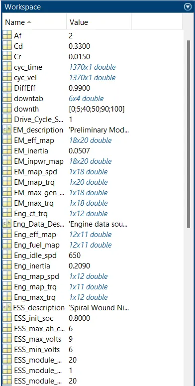
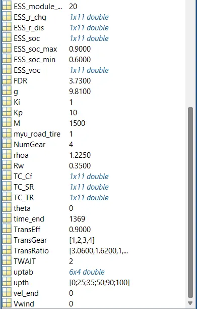
- Code in MATLAB to load all the variables required for running the model in Sumlink.
- Tabulate the fuel economy numbers (kmpl) for UDDS and HWFET cycle and compare these numbers with the baseline numbers for conventional vehicle model.
- To plot the time trace for engine, transmission input, transmission output and wheel speed on one plot.
- To plot engine torque, engine power, fuel rate and fuel consumption using subplots.
- To plot accelerator and brake pedal, gear command, vehicle desired and actual speed, vehicle distance using subplots.
- To plot the engine operating points on the engine fuel map.
- To plot motor speed, torque, motor input power using subplots.
- To plot pack voltage, current and SoC using subplots.
- To plot the motor operating points on the motor input power map, with the motor max motoring and generating torque curves.
THEORY
Conventional Vehicle
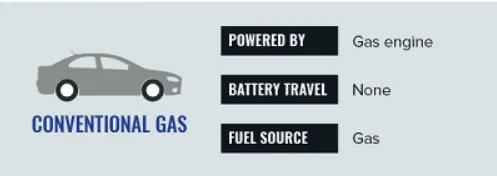
Conventional vehicles are those which use an internal combustion engine fueled by gasoline or diesel to power the wheels. Electricity is used for some accessories such as lights,starter motor,fuel pump etc.., but is not used to move the vehicle.In this vehicle the thermal energy by burning gasoline is converted in to mechanical energy.
Conventional Hybride Vehicle
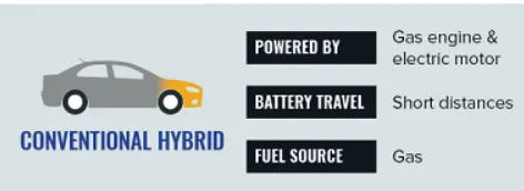
Conventional hybrids, also known as hybrid electric vehicles (HEVs), supports the internal combustion engine with electrical power produced by an on-board electric motor. The electrical system acts as a generator when a driver applies the brakes, converting kinetic energy into electrical energy that is stored in a small battery pack. The primary fuel is gasoline or diesel.
Plug-in Hybrid Vehicle
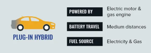
A plug-in hybrid, also called a Plug-In Hybrid Vehicle (PHEV) or an Extended Range Electric Vehicle (EREV), has a larger battery than a conventional hybrid car, and is charged by plugging into an electric outlet. Plug-in hybrids also keep a gasoline or diesel engine as a backup. After the battery energy is exhausted, the engine starts and the vehicle acts like a conventional hybrid until it is plugged in to recharge.
Battery Electric Vehicle
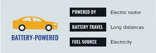
A battery-powered car, or Battery Electric Vehicle (BEV), does not have a gasoline or diesel engine and instead has an electric motor, power electronics, and a battery pack. Battery cars have a longer all-electric range than a plug-in hybrid, but they do not have a fuel backup. Just like a plug-in hybrid, battery-powered cars plug into an electric outlet to refuel.
Types of Hybrid Vehicle Architecture
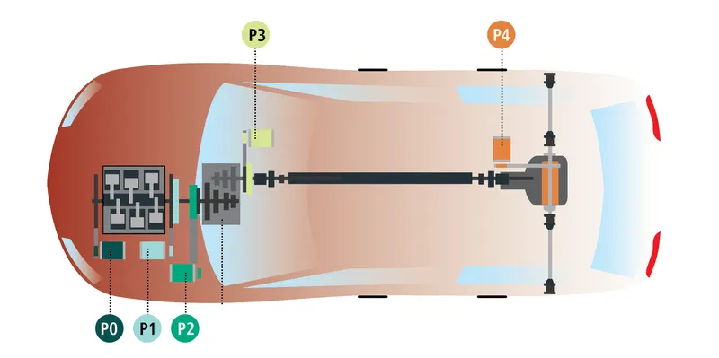
| P0 | The electric machine is connected to the internal combustion engine via a belt on the front-end accessory drive. |
| P1 | The connection between the electric machine and the internal combustion engine is made directly to the crankshaft. |
| P2 | The electric machine is side-attached (through a belt) or integrated between the internal combustion engine and the transmission; the electric machine is decoupled from the ICE and it has the same speed of the ICE (or multiple of it) |
| P3 | The electric machine is connected through a gear mesh with the transmission; the electric machine is decoupled from the ICE and it’s speed is a multiple of the wheel speed |
| P4 | The electric machine is connected through a gear mesh on the rear axle of the vehicle; the electric machine is decoupled form the ICE and it’s located in the rear axle drive or in the wheels hub |
Here we can see in P0 and P1 architectures there is no mechanical disconnection of the electric machine from the engine. On the other hand in P2, P3 or P4 configurations the electric machine disconnects from the engine through a clutch.
- P0 Hybrid/Belt Starter Architecture
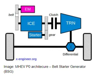
Also know as BiSG from Belt integrated Starter Generator, this mild hybrid topology is the most cost effective due to the limited impact of the 48V system on the existing vehicle architecture.
On a hybrid electric vehicle application, there are two major cost drivers: the impact on the existing powertrain components and the high voltage battery. To minimize the integration costs, the vehicle and transmission architecture should be kept the same as for a conventional vehicle. Thus, the easiest way of achieving a minimum cost is to integrate the 48V electric machine into the already existing engine accessories belt drive, by replacing the 12V alternator (generator).
In the BiSG architecture, the internal combustion engine (ICE) and the electric machine can not be separated, they are mechanically linked through the accessory belt. Therefore, one of the disadvantage of this configuration is that, the engine friction torque will be a parasitic loss for the electric machine when it gives boost torque and when it’s recuperating electrical energy.
- P1 Hybrid /Crankshaft Mounted
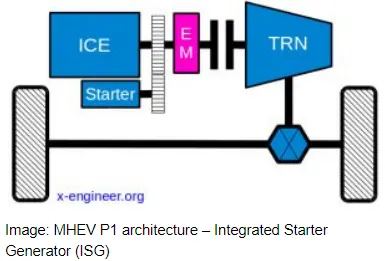
The P1 architecture, with the electric machine connected directly to the crankshaft, is the solution adopted by Honda on their first generation Integrated Motor Assist (IMA) technology. The electric motor functions as a generator, during vehicle deceleration, as an engine starter, and as a motor (to assist the engine) during vehicle accelerations.
One of the biggest advantage of this solution is that the electric motor can provide higher torque than the BiSG, since there is no belt limitation (due to slip). However, since there is no speed / torque ratio between the electric machine and crankshaft, the torque requirements on the electric motor can be quite demanding.
- P2,P3 & P4 Hybrid
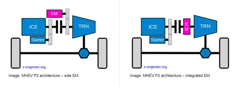
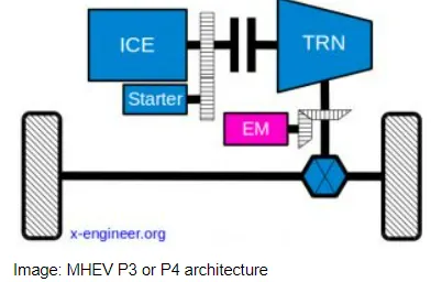
The P2, P3 and P4 mild hybrid architectures are better in terms of energy flow efficiency, mainly because of the positioning of the electric machine. In these types of configurations, the electric machine is positioned after the driveline connecting device (clutch), on the input shaft of the transmission (P2), on the output shaft of the transmission (P3) or on the rear differential (P4).
In the P3 mild hybrid architecture the electric motor is attached on the transmission, on the output shaft. In the P4 architecture, the electric motor is mounted on the rear axle drive or wheel hubs.
The main advantage of the P3 or P4 topology is the highest energy recuperation potential. Compared with the P0, P1 and P2 configurations, the engine and transmission losses, when the driveline is disconnected, are not taken into account during energy regeneration.
The P3 and P4 architectures are have also the potential for electric driving mode (creep) if fitted with a high torque electric machine. The P4 architecture gives the vehicle four-wheel drive capabilities, with the front axle powered by an internal combustion engine and the rear axle powered by an electric motor.
Due to the fact that the electric machine is on the driveline side, for any P2, P3 or P4 architecture, in order to perform engine Stop & Start, another electric machine has to be fitted on the engine side. This function can be achieved with a standard reinforced starter (12 V) or a belt-integrated starter generator (12 V or 48 V).
UDDS Drive Cycle (Urban Dynamometer Drive Schedule)
The UDDS (Urban Dynamometer Driving Schedule) drive cycle is a standardized test procedure used to evaluate the emissions and fuel economy of vehicles. It is one of several driving cycles that have been developed by the U.S. Environmental Protection Agency (EPA) to represent real-world driving conditions. The UDDS drive cycle is designed to simulate the types of driving conditions encountered in an urban setting, such as stop-and-go traffic and short trips.
The UDDS drive cycle consists of a series of stops and starts, accelerations and decelerations, and steady-state driving segments. The cycle begins with a cold start, where the vehicle is allowed to idle for a period of time to allow the engine and catalytic converter to warm up. This is followed by a series of acceleration and deceleration events, designed to simulate the stop-and-go nature of urban driving. The cycle also includes several steady-state driving segments at different speeds, ranging from 20 to 60 mph.
The UDDS drive cycle is typically run on a chassis dynamometer, which is a device that simulates the resistance of driving on a road by applying a load to the vehicle's wheels. The dynamometer is used to measure the vehicle's emissions and fuel consumption during the test. The UDDS drive cycle is used to test light-duty vehicles, including passenger cars, pickup trucks, and vans. It is typically run in conjunction with other driving cycles, such as the Highway Fuel Economy Test (HFET) and the Cold Start FTP (Federal Test Procedure).
The UDDS drive cycle is an important tool for evaluating the environmental performance of vehicles. It allows manufacturers to compare the emissions and fuel economy of different vehicles under controlled conditions and helps regulators ensure that vehicles meet emissions standards. It is also used by consumers to compare the fuel efficiency of different vehicles and make informed purchasing decisions.
HWFET Drive Cycle (Highway Fuel Economy Test)
The Highway Fuel Economy Test (HFET) drive cycle is a standardized test procedure used to evaluate the fuel economy of vehicles. It simulates driving conditions encountered on the highway and consists of acceleration and deceleration events, as well as steady-state driving segments at different speeds. The HFET drive cycle is typically run on a chassis dynamometer, which measures the vehicle's fuel consumption during the test. The cycle is used to test light-duty vehicles and is an important tool for evaluating the fuel efficiency of vehicles. It is used by manufacturers, regulators, and consumers to compare the fuel efficiency of different vehicles and make informed purchasing decisions.
The HFET drive cycle consists of a series of acceleration and deceleration events, as well as steady-state driving segments at different speeds. The cycle begins with a cold start, where the vehicle is allowed to idle for a period of time to allow the engine and catalytic converter to warm up. This is followed by a series of acceleration and deceleration events, designed to simulate the stop-and-go nature of urban driving. The cycle also includes several steady-state driving segments at different speeds, ranging from 35 to 60 mph.
There are two types of Energy modeling approches:
- Forward energy-based fuel consumption model
- Backward Energy-based fuel consumption model
- Forward energy-based fuel consumption model
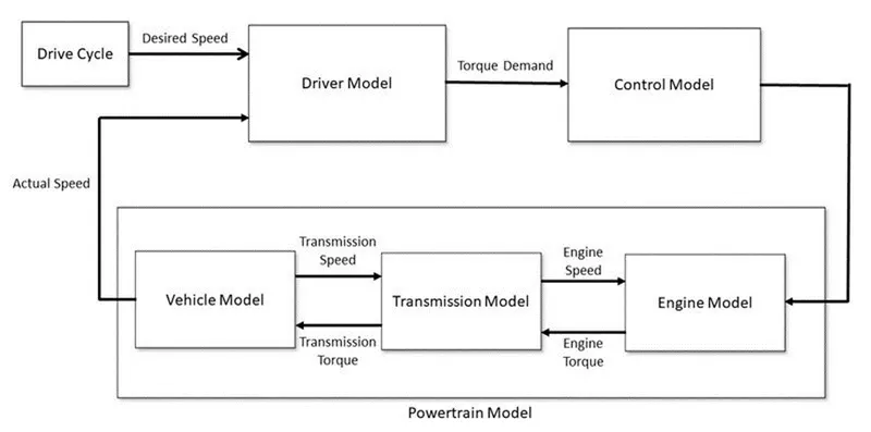
The forward modelling is also known as cause-effect, engine-to-wheel or rear-to-front method. The direction of calculation is the same as the direction of positive power flow which is from engine to wheels.
A forward-facing vehicle model feactures a driver model that provides torque demand in the form of a desiered ICE torque and brake torque, to meet the speed trace from a drivecycle.A basic driver model typically uses one or more Proportional- Intrgral (PI) controllers to achieve the torque demand, with reference to the desiered speed trace.The torque produced by the ICE propagates through the transmission and final drive ratios, before ending up as torque applied at the wheels. This is then exerted to the vehicle mass via force on the tyre contact patch. The vehicle speed that results from the applied force is propagated back through the drivetrain, and returns to the ICE as angular velocity at the crankshaft. Brake torque is applied directly at the wheels.
This model can be used to compare the fuel efficiency of different vehicles, or to identify opportunities for improving the fuel efficiency of a particular vehicle. For example, if you are trying to improve the fuel efficiency of a vehicle, you could modify its design or driving behavior to reduce its energy consumption, and then use the forward energy-based fuel consumption model to estimate the resulting improvement in fuel efficiency.
2. Backward Energy-based fuel consumption model
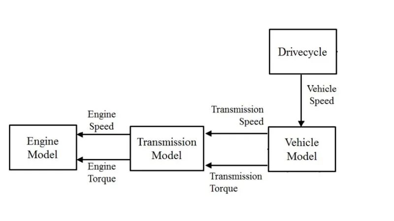
Backward-facing (quasi-static) vehicle model, the ability of the vehicle model to meet the demands of the drivecycle is the principle assumption of a backward-facing model.Based on the speed trace, the resultant force at the tyre contact patch is calculated, where it is converted into wheel torque and propagated back to the ICE via the drivetrain, along with angular velocity. As a result, there is no driver model present. With both speed and torque imposed onto the powertrain components, a backward-facing model can also be considered as non-causal (physically non-realisable).During the optimisation routine, the powertrain component sizing is determined by the ability of the component to address both the speed and torque imposed on the component (i.e. the power requirements).
Backward-facing models rely on efficiency maps that were created based on torque and speed data, and usually produced during steady-state real world testing. This results in the calculation being relatively simpler than forward-facing models (essentially lookup tables instead of state equations),and can therefore be run over relatively larger time steps.Unfortunately, the very nature of using steady state maps hinders the performance of backward-facing models when it comes to representing dynamic effects.
PROGRAM CODE
%%%%%%%%%%%%%%%%%%%%%%%%%%%%%%%%%%%%%%%%%%%%%%%%%%%%%%%%%%%%%%%%%%%%%
%% Skill-Lync -> Hybrid Drives Development
% Project 2 - P1 Hybrid Vehicle Model
% By - Anjith VS

clear all
close all
clc
%% Vehicle Parameters
M = 1500;       % Vehicle weight [kg]
Cr = 0.015;     % Rolling resistance coefficient
Rw = 0.35;      % Rolling radius [m]
Cd = 0.33;      % Drag coefficient
Af = 2;         % Frontal area [m2]
rhoa = 1.225;   % Air density [kg/m3]
Vwind = 0;      % Wind velocity [kmph]
g = 9.81;       % Gravitational acceleration [m/s2]
theta = 0;      % Slope [deg]
myu_road_tire = 1; % Coefficient of friction between tire - road interface

%% Powertrain Parameters
FDR = 3.73;                         % Final Drive Ratio / Diff Ratio
DiffEff = 0.99;                     % Differential efficiency (assumed independent of operating conditions)

NumGear = 4;                        % Number of gears in transmission
TransGear = [1:NumGear];            % Transmission Gears
TransRatio = [3.06, 1.62, 1, 0.7];  % Corresponding Transmission ratios
TransEff = 0.90;                    % Transmission efficiency (assumed independent of operating conditions)

TC_SR = [0, .5, .6, .7, .8, .87, .92, .94, .96, .97, 1];   % Torque Converter Speed Ratio (Matlab default) -> TurbSpd/PumpSpd
TC_TR = [2.232, 1.5462, 1.4058, 1.2746, 1.1528, 1.0732, 1.0192, 1, 1, 1, 1];   % Torque Converter Torque Ratio (Matlab default) -> TurbTrq/PumpTrq
TC_Cf = 1e-4 * [.72558, .66322, .63463, .59042, .51331, .4144, .29287, .22444, .12186, .04386, 0]; % Torque Converter Capacity Factor (Matlab default) -> PumpTrq/PumpSpd^2 [Nm/rpm^2]

load Vehicle_Data/Engine_data_1_9L_Saturn_95kW
load Vehicle_Data/Trans_Shift_map
load Vehicle_Data/EM_Honda_Insight_10kW
load Vehicle_Data/ESS_NiMH6


ESS_init_soc = 0.8;
ESS_soc_max = 0.9;
ESS_soc_min = 0.6;


%% Driver Parameters
Kp = 10;                    % P gain for driver PI model
Ki = 1;                     % I gain for driver PI model
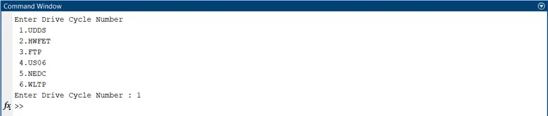
fprintf('Enter Drive Cycle Numbern 1.UDDSn 2.HWFETn 3.FTPn 4.US06n 5.NEDCn 6.WLTPn'); % Drive cycle selection
Drive_Cycle_Select =input('Enter Drive Cycle Number : ');

% Drive cycle values in m/s

if Drive_Cycle_Select == 1
    load DriveCycles/UDDS;

elseif Drive_Cycle_Select == 2
    load DriveCycles/HWFET;

elseif Drive_Cycle_Select == 3
    load DriveCycles/FTP;

elseif Drive_Cycle_Select == 4
    load DriveCycles/US06;

elseif Drive_Cycle_Select == 5
    load DriveCycles/NEDC;

elseif Drive_Cycle_Select == 6
    load DriveCycles/WLTP;

end

time_end = cyc_time(end);
vel_end = cyc_vel(end);
CODE EXPLAINATION
- The program begins by clearing and closing the memory using close all clear all clc functions.
- Then the vehicle parameters and constants were initilized.
- The engine datas and the gear shift datas were loaded to Matlab using the load command.
- Then the driver parameters proportional and integral cofficients were decelared.
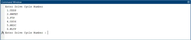
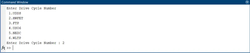
- Then using the fprintf() the different drive cycles were showen and using the input() command the user input of the required drive cycle is recieved.
- Again using load command the particular drive cycle data selected by user is loaded in Matlab and the end time and end velocity of vehicle is obtained.
COMMAND WINDOW
Taking user input
WORKSPACE
SIMULINK MODEL
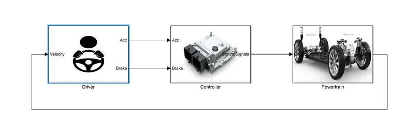
The Simulink model for the convection vehicle consist of using 3 main subblocks: driver model, control model and powertrain block.The model developed is capable to simulate the vehicle on different drive cycles like UDDS, HWFET, FTP, US06,NEDC and WLTP.
The Solver is selected to be Fixed-step ode3 solver and the stimulation end time were adjusted to the drive cycle selected.
1. The Driver model
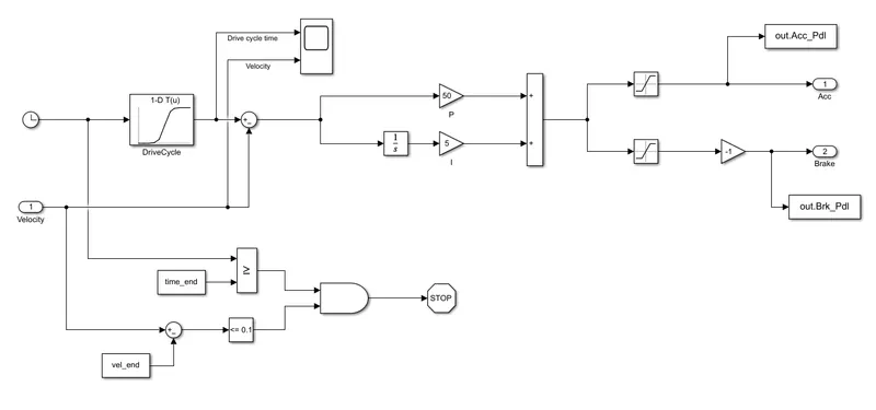
- The driver block is the staring stage of the model as in real the driver is the one who controls the vehicle according to the surrounding driving conditions and his own needs.
- Insteas of using a real driver we stimulate the driver using different type of drive cycles.
- The drive cycle is a Velocity vs Time charts that is based on certain driving conditions like city driving,highway driving,fuel economy driving etc..
- The Driver Model is a basicially a Proportional Integral (PI) controller that generates accelerator and brake pedal outputs to match the desired and actual vehicle speeds as per the drive cycle.
- The PI controller controls the error between the required drive cycle velocity and actual vehicle velocity so as to make both the drive cycle and actual vehicle velocity same.
- The top speed of the vehicle is limited to 100 kmph and also the decclearation using the saturation block.
- This model takes in the vehicle velocity and gives the accleration and brake output to controller.
- A scop block is used to monitor the Drive cycle
2. Controller model
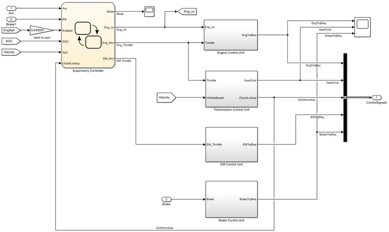
- The controller as the name suggest control every components in the model, it is the brain of the model.
- It takes in all the current conditions like accleration,break,engine speed,SOC of battery,Velocity and the clutch lockup values and then analyse it and provide output to each contorllers to perform as desiered.
- The Controller block has 4 controller : Engine control unit, Transmission Control unit, Electric Motor Control unit and the Brake Control unit.
- All the control units are supervised or controlled by a Supervisory control unit.
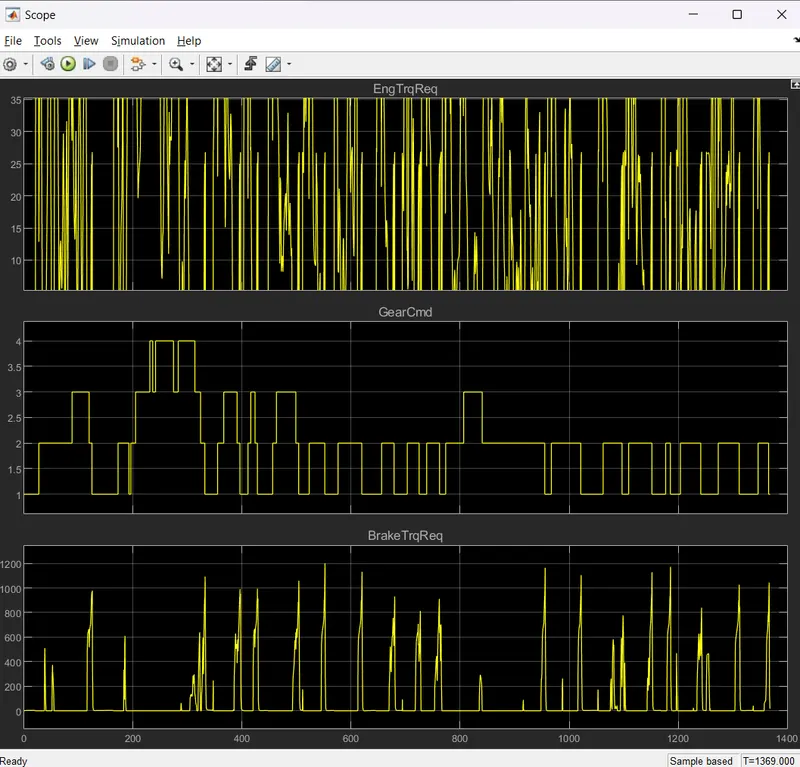
- Two scop blocks were used here to monitor the Mode shifting and Engine torque required, Gear command and Bake Torque required.
- All the output of this block is fed to the 'bus creator' which will be fed to the power train as control signal.
2. a. Supervisory Controller
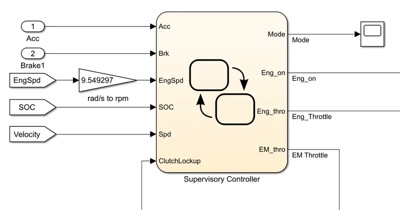
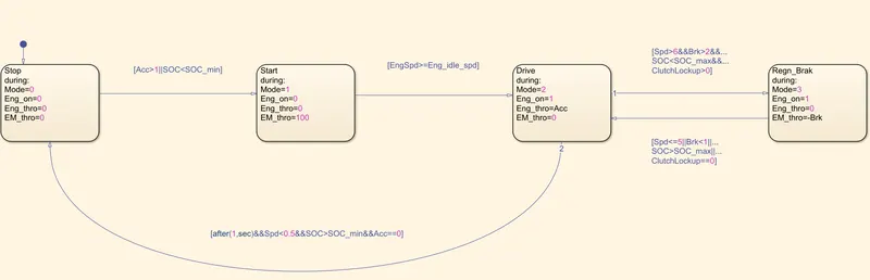
- The supervisory controller is modeled using State flow.
- The chart takes in Accleration, Brake, Engine speed, SOC, Velocity, Clutch lockup values and depending on the conditions modeled inside the chart block it gives out the when all the engine should be kept on, what should be engine throttle and what should be the Electric motro throttle.
- The supervisory controller shifts between 4 modes : Stop, Start, Driving and Regeneration mode.
- It analyse and decide when to give the electric motor input and when to keep the engine on and off and when to do the regeneration while breaking.
2. b. Engine Control Unit
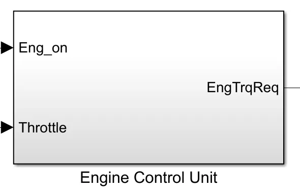
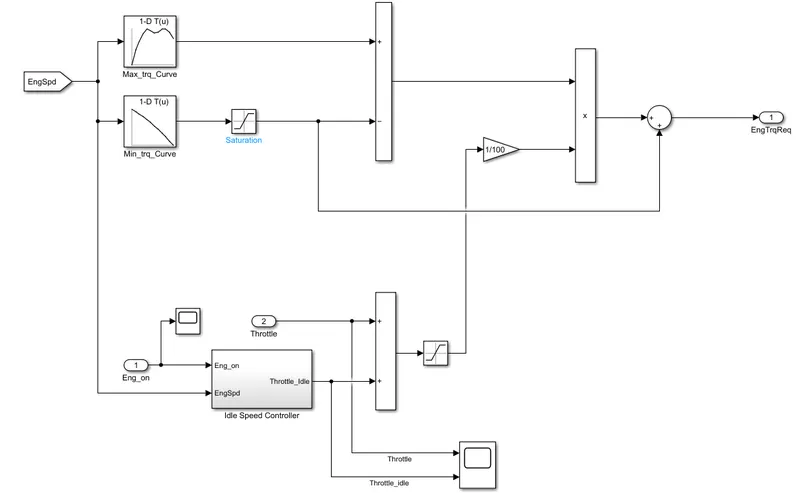
- The inputs to this unit are Engine speed and engine on/off .
- Since this is a hybrid vehicle, the engine can be shut off during idling or low power applications.
- The Engine speed is fed to the lookup tables which will gives required torques both positive and negative to meet the vehicle demand.
2. b. i) Idle Speed Controller
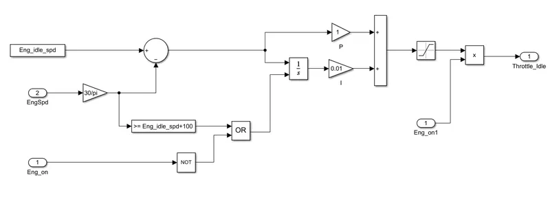
- The Idle Speed Controller is the subsystem of the Engine controller which will takes in engine speed engine on/off state.
- It is this contoller that controls engine idle throttle when the engine is in on condition.It will also reset the integrator block after each engine on/off.
2. c. Transmission Control Unit
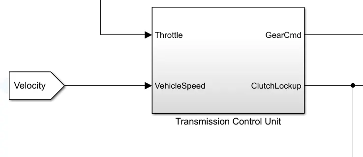
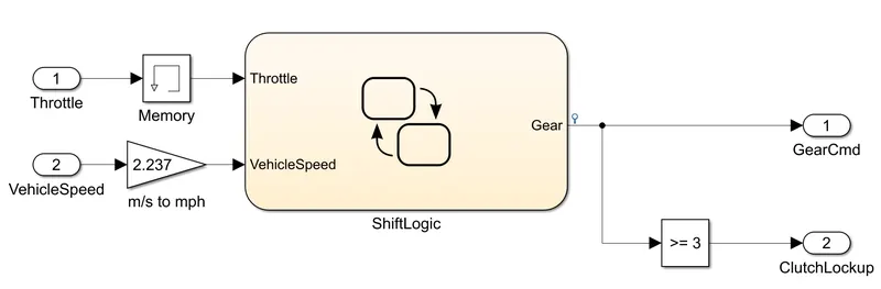
- The transmission control unit takes in the Throttle which is provided from the supervisory controller and the Vehicle speed which is fed using a from block.
- Based on this input the shift logic block will calculate to which gear to shift for getting optimum efficienc.
- The shift logic block gives the gear command and the clutch lockup value.
- Since the model has a automatic transmission by using torque converter, the shift logic block decides when to lockup the clutch so that the power flows directly whenever the vehicle requires less power.
- Here the clutch lockup is set as for gears more than 3rd gear.
2. c. i) Shift Logic Chart
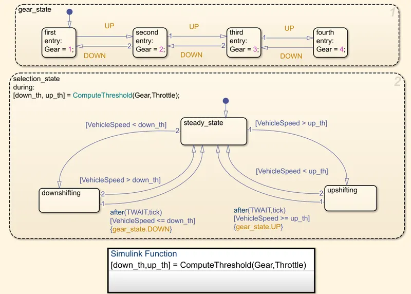
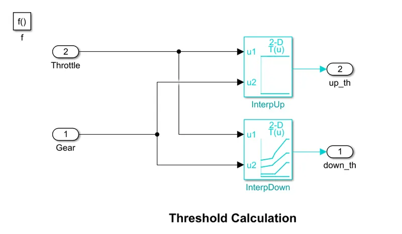
- The shift Logic is a State flow chart which is used to decide to which gear to shift to.
- The shifting of gears are done by calculating the vehicle speed.
- The shifting will takes place up and down depending on the speed value.
2.d. EM Control Unit
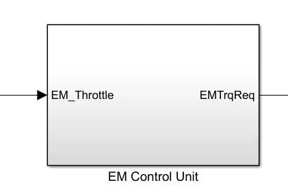
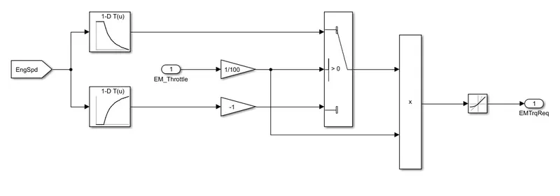
- EM control unit controls the torque required by the vehicle.
- The block takes in the throttle required by the vehicle which it get form the supervisory controller.
- Since the Electric motor is a P1 hybrid it is mounted directly on the crank shaft, the input of the motor is the engine speed itslef.
- Using the lookup tables and the engine speed the model gives out the required torque which is to be generated by the electric motor.
2. e. Brake Control Unit
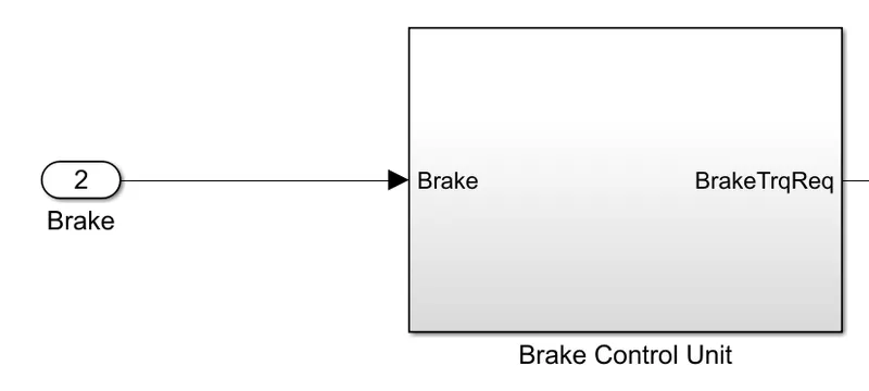
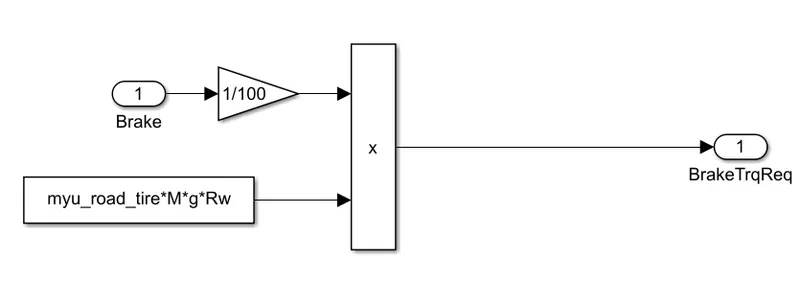
- The Brake contorl unit controls the Brake torque required by the vehicle.
- It takes in the brake peddal value applied and depending on this input and the Rolling resistance force, the controller gives out the amount of brake torque required to meet the braking demands.
3. Power train
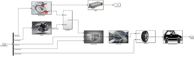
- The power to move the vehicle is obtained form here.
- All the out from the controller block is decoded from the control signal using a bus Selector.
- The block consist of Electric motor, Engine, Crank hub, Transmission, Differential, Wheels, Energy Storage System(ESS) and Vehicle Dynamics.
- The output of this block is the velocity of the vehicle and SOC of battery pack.
3. a. Electric Motor
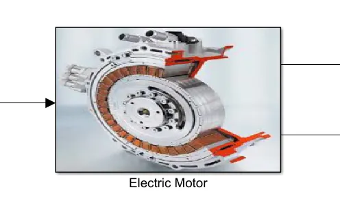
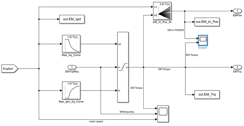
The Electric Motor take in the Troque requirement froom the controller block and dependig on the engine speed (which is the motor speed itslef), it produces torque and power required.
The motor power is required to draw the power form the battery pack as the motor keeps on working.
This is done using speed - torque lookup tables.
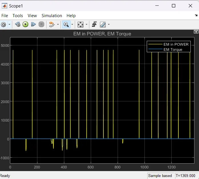
Two scop blocks are used here one is to monitor the motor speed and the Motor torque required Torqeu given and the other to monitor the power drawn and the torque generated.
3. b. Engine
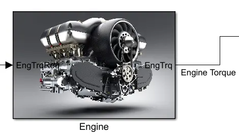
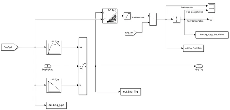
- Similar to electric motor the engine takes in the engine required torque and produces the torque as per requested to the crank hub.
- Using the dynamic saturation block and the lookup tables the maxium and minium torque that the engine can produce is given to the crank hub.
- Inorder to swith off the fuel flow the engine on input is used once the engine is off it will shut the fuel flow.
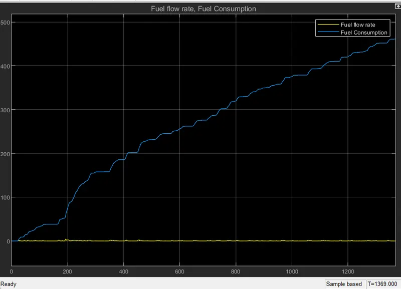
- A scop block is used to monitor the fuel flow rate and the fuel consumption.
- Inorder to keep the fuel flow rate to be positive always a saturation block is used.
3. c. Crank hub
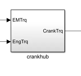
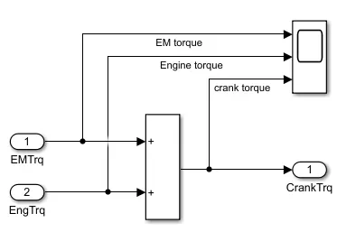
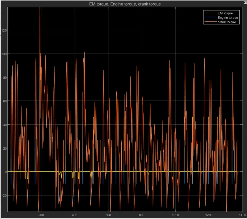
- The crank hub takes in the engine torque and the electric motor torque and it adds up.
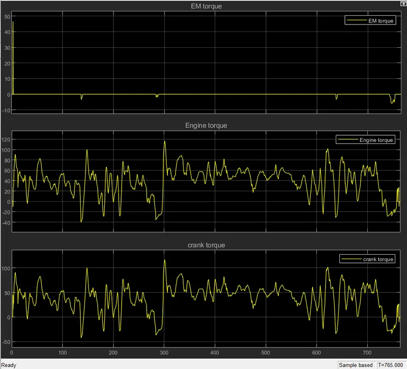
- The crank torque is the sum of engine torque and the engine torque.
- A scope block is used to monitor the electric motor torque, engine torque and the crank torque.
3. d. Transmission
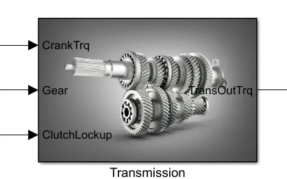
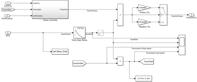
The transmission block consists of the Torque converter and the Transmission output shaft.
The torque converter takes in the crank torque and clutch lockup values and also the transmission input speed and gives out the transmission input torque.
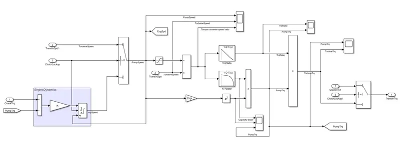
- Inside the torque converter, the torque coming from the crankshaft is scaled up or down primarily based on the requirements at the wheels.
- In case if the vehicle is moving uphill, the torque demanded by using the car in such times is high. subsequently, the torque converter desires to scale up the crank torque.
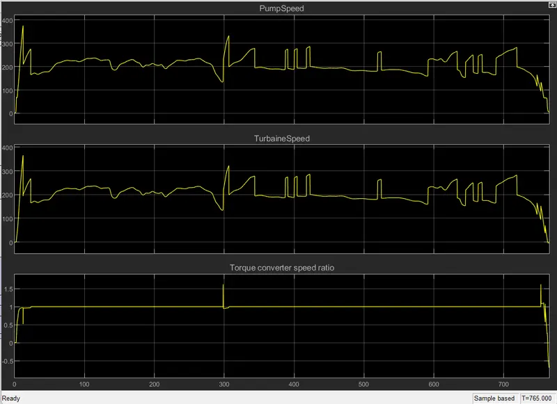
- The torque converter is a separate subsystem in transmission,the inputs to it are the crank torque, transmission input velocity and the clutch lockup condition.
- The difference between the new generated crank torque and the previous pump torque is the error that the torque converter needs to correct. The pump speed is obtained by dividing the inertias of the engine and motor.
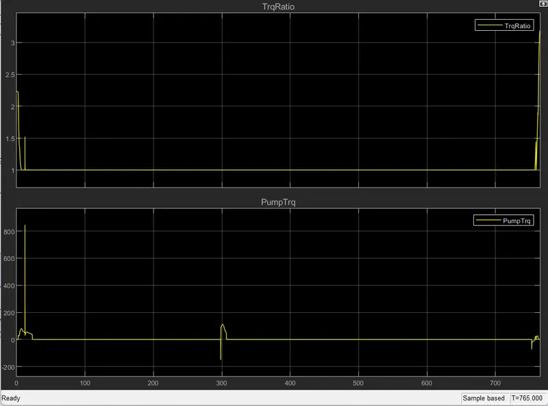
- The turbain speed is determined by the clutch lookup status and using the torque ratio and K-factor lookup maps, the turbine torque is estimated and acts as the input torque to the transmission shaft.
3. e. Differential
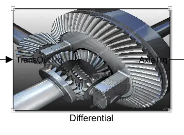
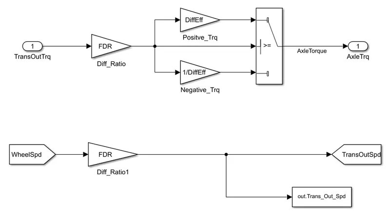
- The differential block distributes the torque between the driving wheels.
- A swithch block is used to provide the positive and negative axel torque.
- The block takes in the transmission output torque and gives out the axel torque.
- Also the transmission output speed is obtained by multiplying wheel speed with the differential ratio.
3. f. Wheels
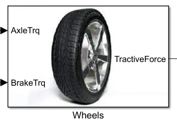
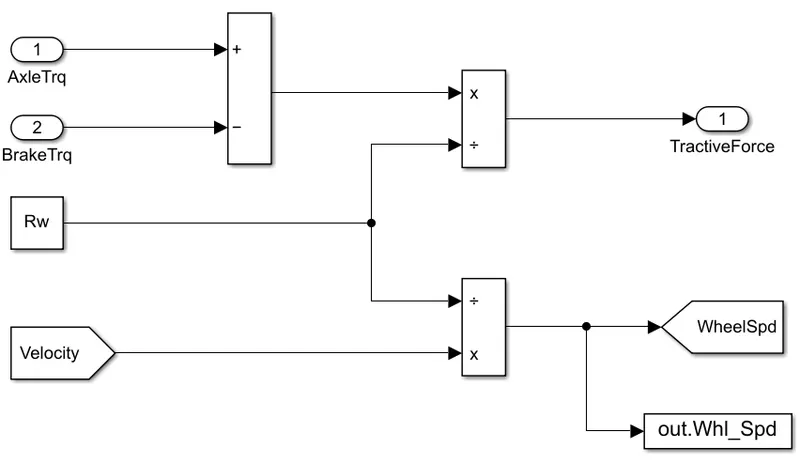
- The block takes in the axle torque from the differential block and the brake torque signal from the controller and it is then added and divided with the Rolling radius of the wheel.This will provide the Tractive force on the wheel.
- It is also used to get the wheel speed of the vehicle by taking in the velocity and dividing with the rolling radius of the wheels.
3. g. Vehicle Dynamics
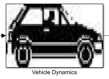
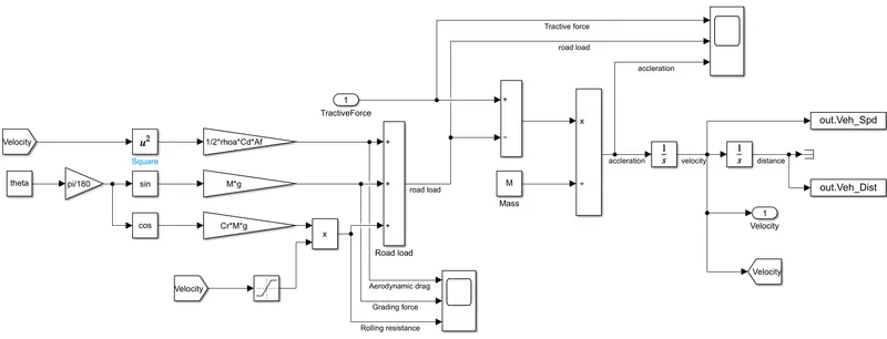
- This block is used to find the velocity of vehicle after overcoming the rolling resistance, aerodynamic drag, grading resistance and inertial resistance which will make up the road load.
- It is then divided with the mass of the vehicle and integrated to get the velocity of the vehicle.
3. h. ESS ( Energy Storage System)
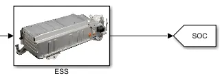
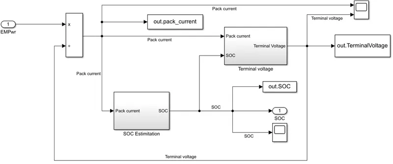
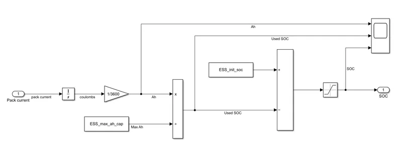
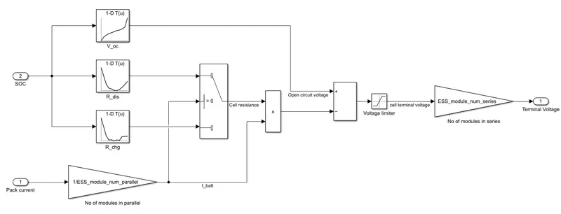
- The ESS is the energy storage for the electric motor and is used to find the SOC and also the terminal voltage and pack current of the battery pack.
- It takes in the Electric motor power used by the motor and also store the energy during regenerative braking.
- The battery pack also has to maintain its state of charge whenever it goes below Charge sustaining mode in HEVs.
- Here the threshold SOC is set to be 60%
OUTPUT (UDDS Drive Cycle)
Drive cycle velocity vs Vehicle velocity of UDDS drive cycle from driver block :
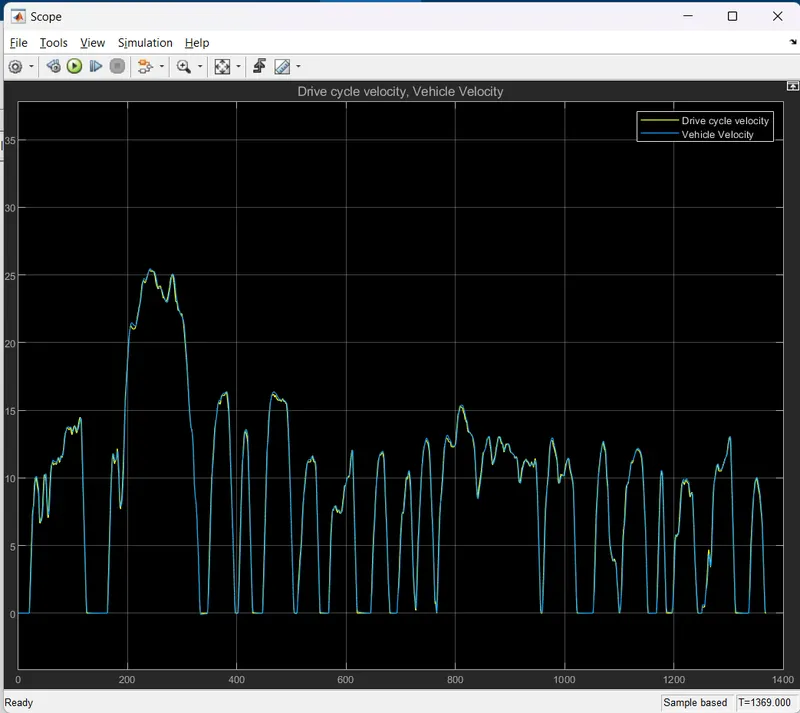
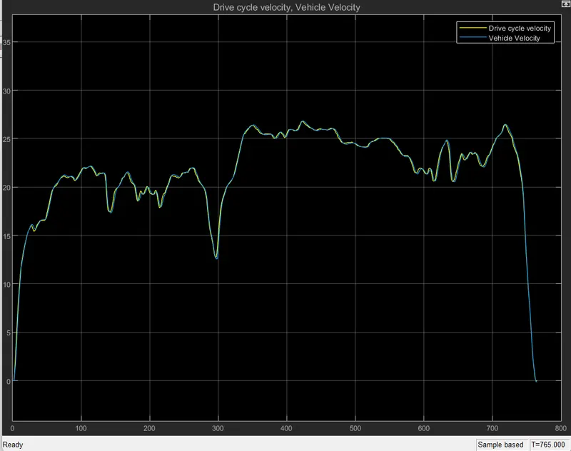
- From the scope it is clear that the actual velocity and the cycle velocity had close resemblance.
- The stimulation time was change to 1400 seconds for better view.
Scope of Mode Shifting by the supervisiory controller in UDDS Drive cycle :
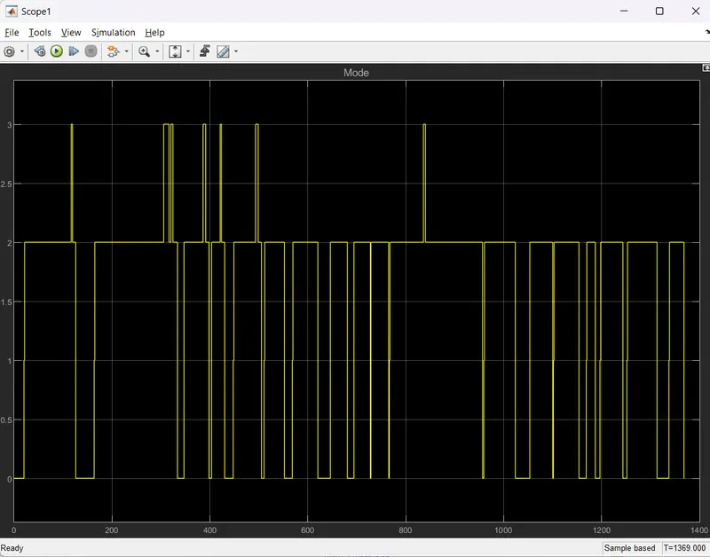
- Here we can see the shifting between the three modes by the supervisory controller with respect ot time.
- By counting the mode 3 values in the scop it is found that the regen has done 7 time in the entire cycle.
Engine Torque Gear command and Break torque output in UDDS Cycle :
Engine On Scop in UDDS Drive Cycle :
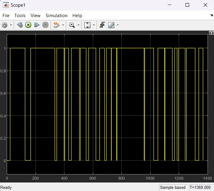
- This scope shows at which all times the engine is set to on and whenever it is kept to off position.
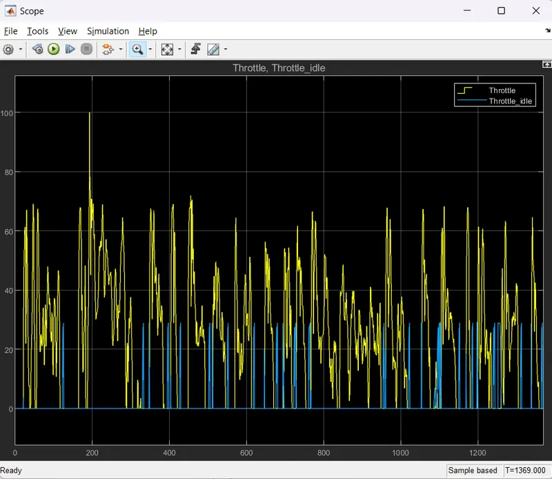
The Throttle and Idle Throttle Scop in UDDS Drive Cycle
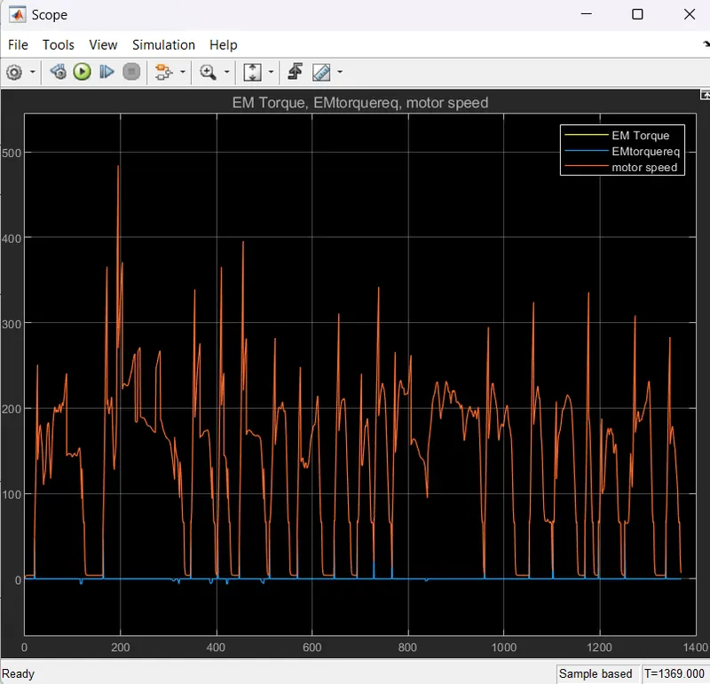
The Motor speed, EM Required torque and Torque provided in UDDS Drive Cycle :
EM input power and EM Torque in UDDS Drive Clcle :
Fuel flow rate and Fuel consumption in UDDS Drive Cycle with time :
Electric motor torque,Engine torqeu and Crank torque in UDDS Drive cycle :
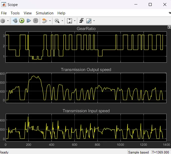
Gear ratio, Transmission output speed and Transmission input speed in UDDS Drive cycle :
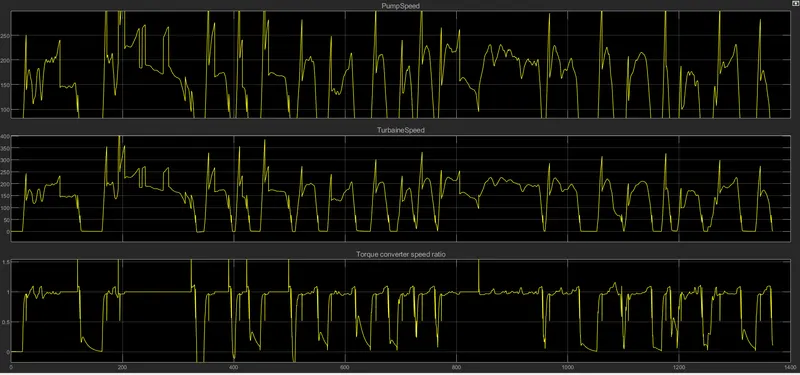
Pump Speed,Turbine Speed ,Torque converter speed ratio from Transmission block in UDDS Cycle
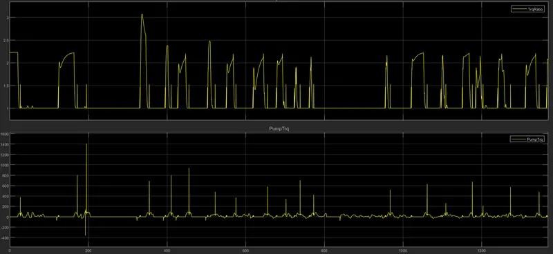
Torque ratio and Pump Torque from Transmission block in UDDS Cycle :
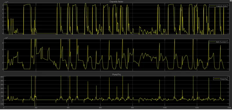
Capacity Factor Pump Torque from Transmission block in UDDS Cycle :
Aerodynamic drag,Grading force and Rolling resistance VS Time from Vehicle dynamic block in UDDS Cycle :
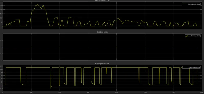
- From the graph it is clear that the vehicle is travelling on flat road because of whcih the grading force is zero in the entire cycle.
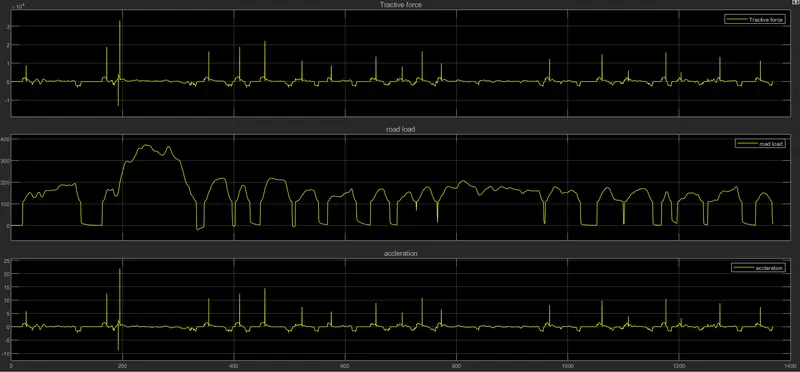
Tractive force,Road load and Accleration VS Time From vehicle dynamic block in UDDS Cycle :
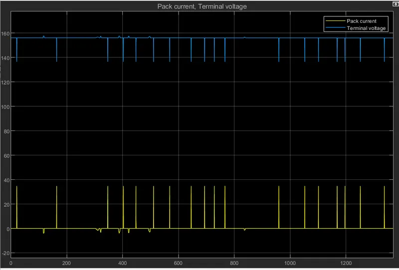
Pack Current and Terminal voltage scope for UDDS Drive Cycle
Ampere hour,SoC and Used SoC scope druing UDDS Drivr Cycle :
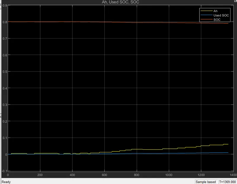
SOC scope of UDDS Drive Cycle
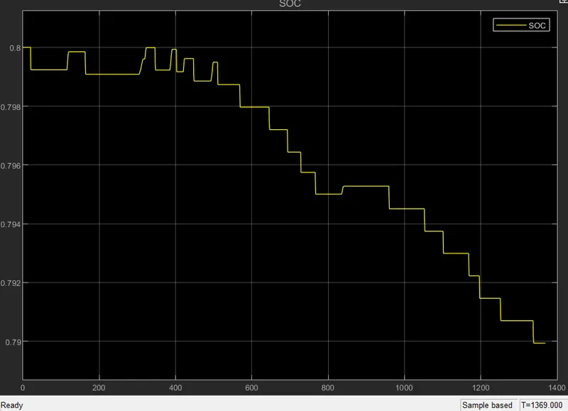
- We can see that the SOC is dropping from the initial state and regen is happening rarely
OUTPUT (HWFET Drive Cycle)
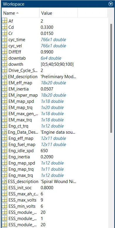
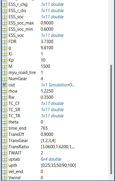
Workspace
Drive cycle velocity vs Vehicle velocity of HWFET drive cycle from driver block :
Scope of Mode Shifting by the supervisiory controller in HWFET Drive cycle :
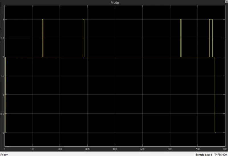
- Only 4 Regen happened
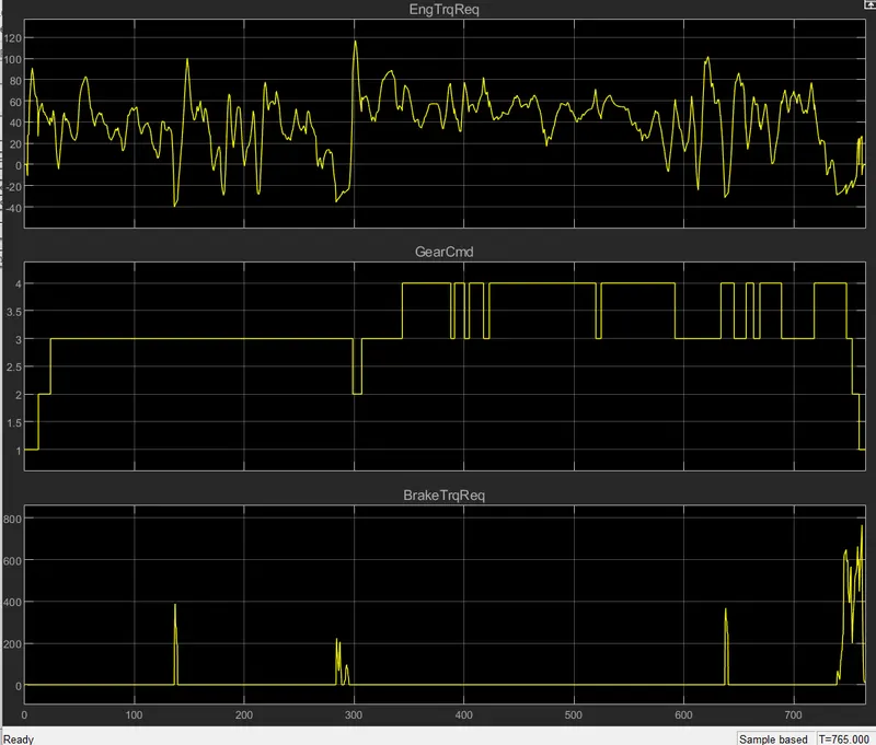
Engine Torque Gear command and Break torque output in HWFET Cycle :
Engine On Scop in HWFET Drive Cycle :
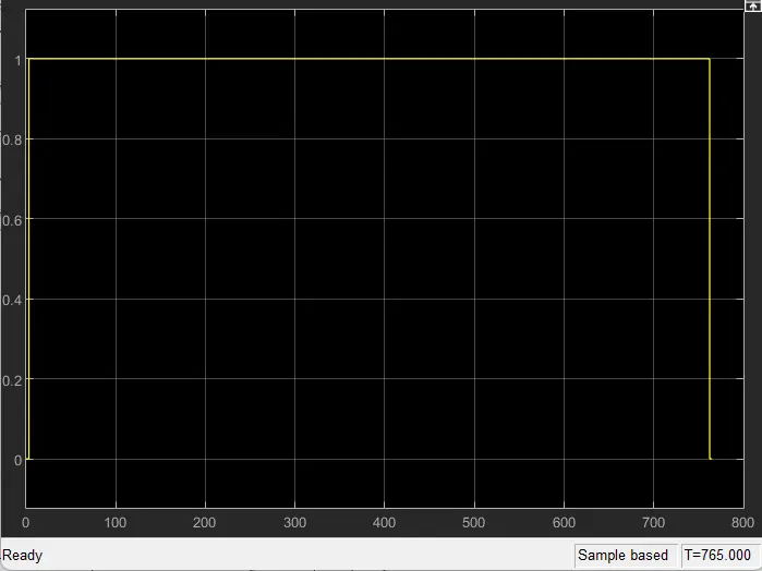
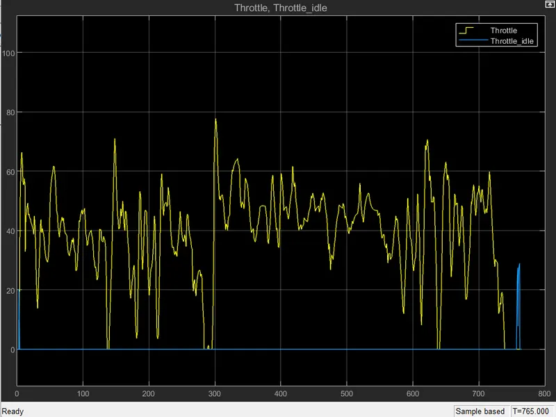
- Here we can see the engine is kept on throughout the entire drive cycle where as in UDDS Cycle the there were frequent ON and OFF of engine.
The Throttle and Idle Throttle Scop in HWFET Drive Cycle :
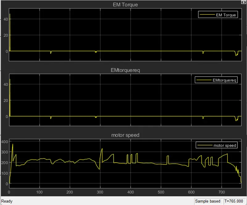
The Motor speed, EM Required torque and Torque provided in HWFET Drive Cycle :
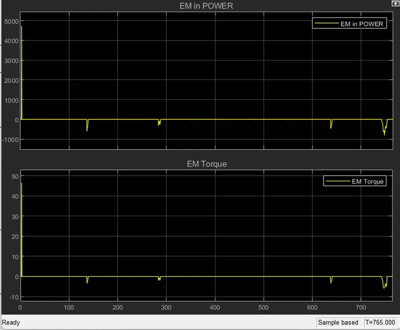
EM input power and EM Torque in HWFET Drive Clcle :
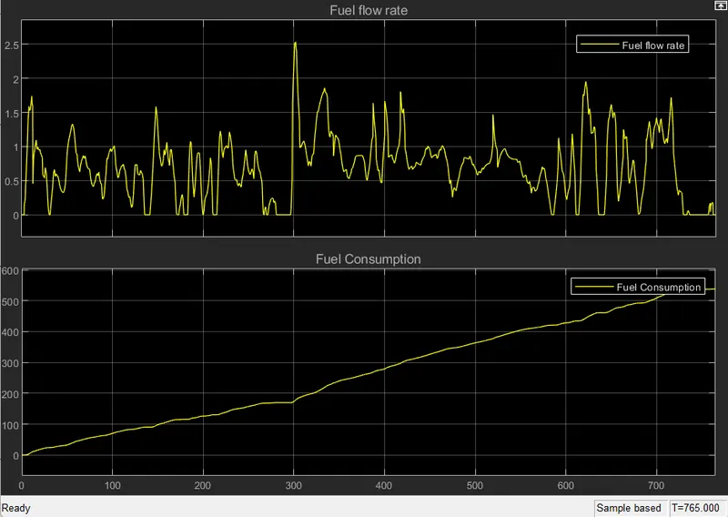
Fuel flow rate and Fuel consumption in HWFET Drive Cycle with time :
Electric motor torque,Engine torque and Crank torque in HWFET Drive cycle :
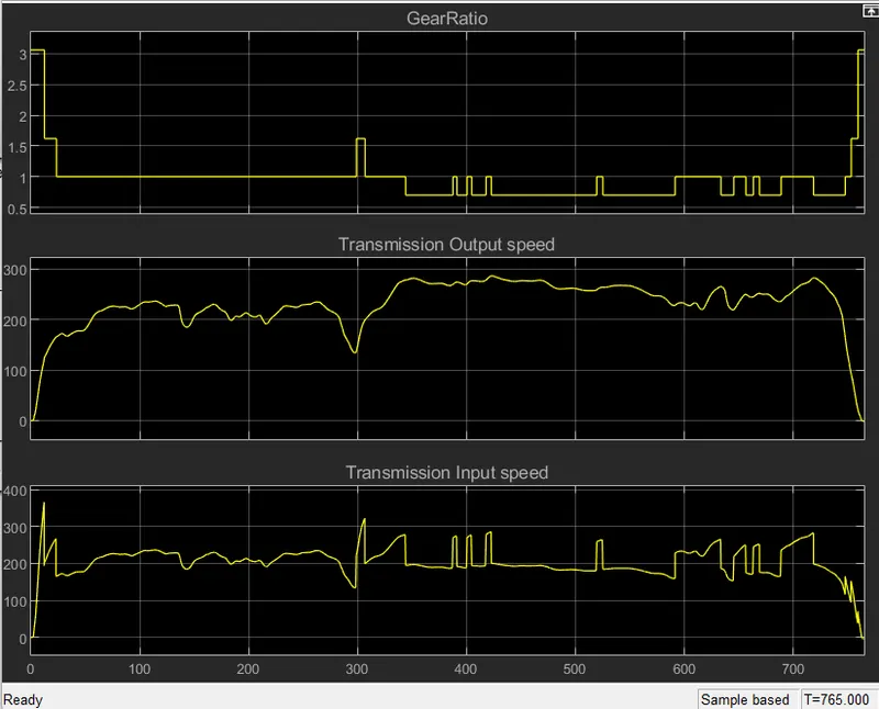
Gear ratio, Transmission output speed and Transmission input speed in HWFET Drive cycle :
Pump Speed,Turbine Speed ,Torque converter speed ratio from Transmission block in HWFET Cycle :
Torque ratio and Pump Torque from Transmission block in HWFET Cycle :
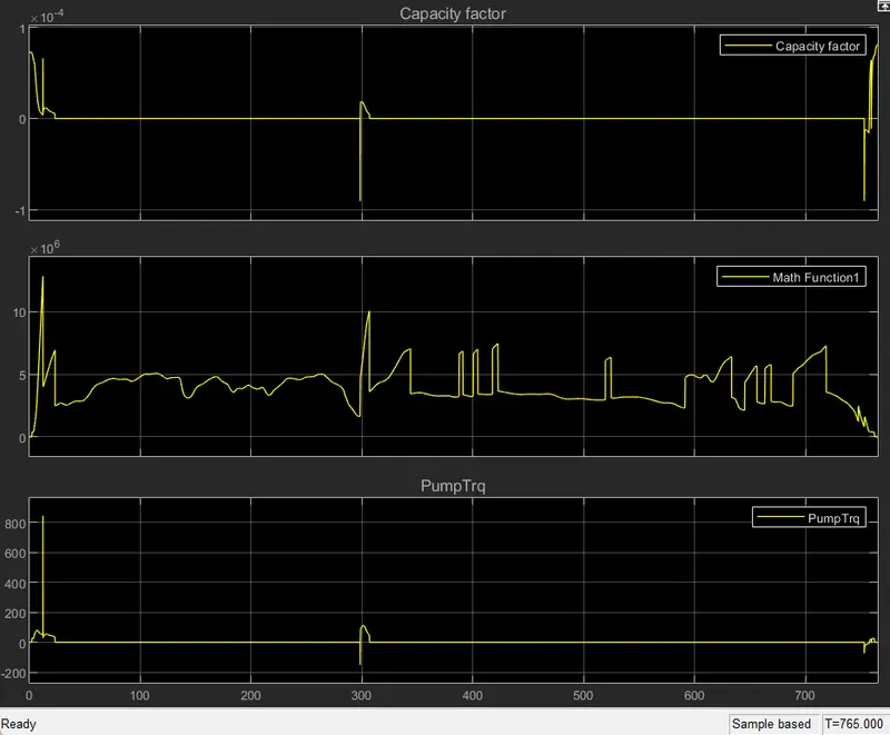
Capacity Factor, Pump Torque from Transmission block in HWFET Cycle :
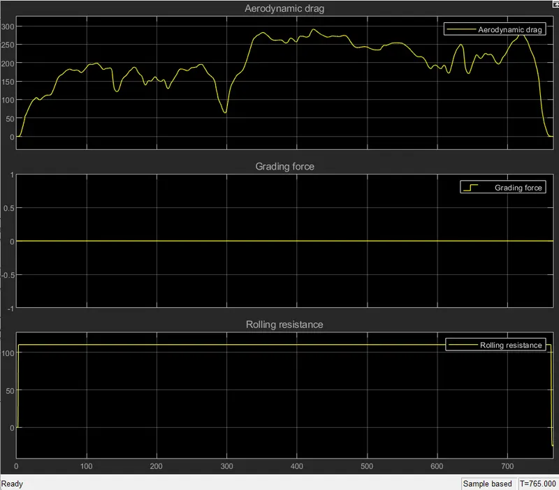
Aerodynamic drag,Grading force and Rolling resistance VS Time from Vehicle dynamic block in HWFET Cycle :
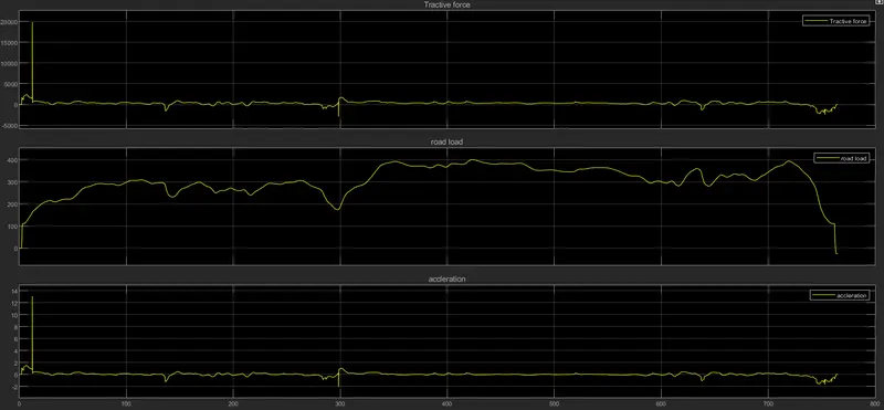
Tractive force,Road load and Accleration VS Time From vehicle dynamic block in HWFET Cycle :
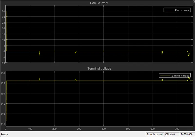
Pack Current and Terminal voltage scope for HWFET Drive Cycle :
Ampere hour,SoC and Used SoC scope druing HWFET Drivr Cycle :
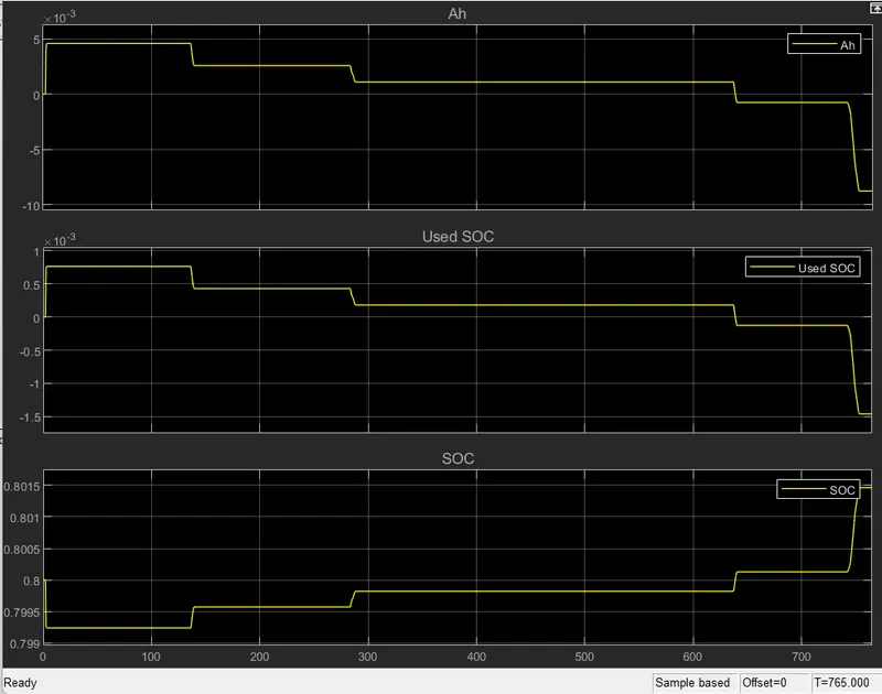
SOC scope of HWFET Drive Cycle :
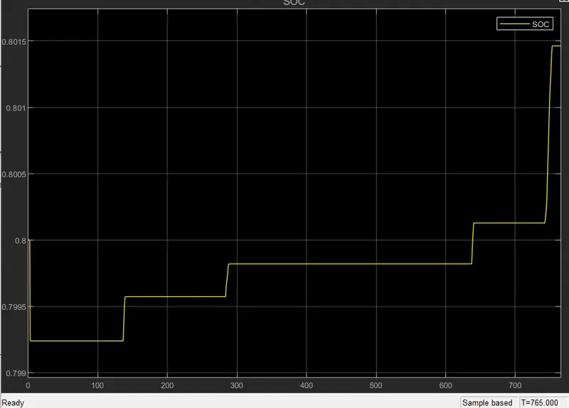
- In this scope we can find a drastic change form that we saw in UDDS deive cycle.
- In UDDS the SOC was gradually decreasing, but in HWFET the SOC went down quickly and then stated to gain charge.
- This shows that the regen is high in HWFET
Post-Processing P1 Hybrid Vehicle in simulation model
PROGRAM CODE
% Post Processing
% Renaming & Defining Variables
Time = out.tout;
Acc_Pdl = out.Acc_Pdl;                      % Accelerator pedal [%]
Brk_Pdl = out.Brk_Pdl;                      % Brake pedal [%]
Gear_Cmd = out.Gear_Cmd;                    % Transmission gear
Trans_In_Spd = out.Trans_In_Spd*30/pi;      % Transmission input speed [rpm]
Trans_Out_Spd = out.Trans_Out_Spd*30/pi;    % Transmission output speed [rpm]
Eng_Trq = out.Eng_Trq;                      % Engine brake torque [Nm]
Eng_Spd = out.Eng_Spd*30/pi;                % Engine speed [rpm]
Eng_Fuel_Consump = out.Eng_Fuel_Consumption;% Engine fuel consumption [g]
Veh_Dist = out.Veh_Dist/1000;               % Distance traveled by vehicle [km]
Veh_Spd = out.Veh_Spd*18/5;                 % Vehicle speed [kmph]
Whl_Spd = out.Whl_Spd*30/pi;                % Wheel speed [rpm]
Eng_Fuel_Rate = out.Eng_Fuel_Rate;          % Engine fuel rate [%]
Desiered_velocity = cyc_vel*18/5;           % Desiered velocity as per drive cycle [kmph]
EM_trq = out.EM_Trq;                        % Electric Motor Torque [Nm]
EM_spd = out.EM_spd;                        % Electric Motor Speed [rpm]
EM_In_Pwr = out.EM_In_Pwr;                  % Electric Motor Power [W]
TerminalVoltage = out.TerminalVoltage;      % Terminal voltage of battery [V]
pack_current=out.pack_current;              % Pack current[I]
SOC=out.SOC;                                % State of charge [%]

% Data analysis
Eng_Pwr = (Eng_Spd.*Eng_Trq)/.1000;                          % Engine brake power [kW]
rho_petrol = 0.7197;                                         % Density of petrol [kg/L]
kmpl = Veh_Dist(end)/(Eng_Fuel_Consump(end)/1000/rho_petrol);% Fuel economy [kmpl]

% Tabulation of Average speed and Fuel econony
Avg_speed = sum(Veh_Spd)/length(Veh_Spd);
table(Avg_speed,kmpl(:,1),'VariableNames',{'Average Speed [kmph]','Fuel Economy [kmpl]'})

% Plotting

% Time trace for engine, transmission input, transmission output and wheel speed
figure(1)
hold on
grid on
plot(Time,Eng_Spd,'LineWidth',1,'Color','b');
plot(Time,Trans_In_Spd,'LineWidth',1,'Color','m');
plot(Time,Trans_Out_Spd,'LineWidth',1,'Color','k');
plot(Time,Whl_Spd,'LineWidth',1,'Color','g');
xlabel('Time [s]');
ylabel('Speed [rpm]');
xlim([0, Time(end)]);
legend('Engine Speed','Transmission Input Speed','Transmission Output Speed','Wheel Speed');

% Engine torque, engine power, fuel rate and fuel consumption
figure(2)
subplot(2,2,1);
plot(Time,Eng_Trq,'linewidth',1,'color','1,0.7,0.3');
xlabel('Time [s]');
ylabel('Engine Torque [Nm]');
title('Engine Torque VS Time');
grid on;
subplot(2,2,2)
plot(Time,Eng_Pwr,'linewidth',1,'color','0.8,0.3,0.6');
xlabel('Time [s]');
ylabel('Engin Power [Kw]');
title('Engine power VS Time');
grid on;
subplot(2,2,3)
plot(Time,Eng_Fuel_Rate,'linewidth',1,'color','0.4,0.7,0.5');
xlabel('Time [s]');
ylabel('Engin fuel rate [%]');
title('Fuel rate VS Time');
grid on;
subplot(2,2,4)
plot(Time,Eng_Fuel_Consump,'linewidth',1,'color','0.6,0.2,1')
xlabel('Time [s]');
ylabel('Fuel Consumption [g]');
title('Fuel Consumption VS Time');
grid on;

% Accelerator and brake pedal, gear command, vehicle desired and actual speed, vehicle distance
figure(3)
subplot(4,1,1)
hold on
grid on
plot(Time, Acc_Pdl, 'linewidth', 1, 'Color', 'g');
plot(Time, Brk_Pdl, 'linewidth', 1, 'Color', 'b');
ylabel('Pedal [%]');
xlim([0, Time(end)]);
legend('Accel','Brake');

subplot(4,1,2)
hold on
grid on
plot(Time, Gear_Cmd, 'linewidth', 1, 'Color', '0.4,0.8,1');
xlim([0, Time(end)]);
xlabel('Time [s]');
ylabel('Gear');

subplot(4,1,3)
hold on
grid on
plot(Time,Veh_Spd,'linewidth',1,'Color','black');
plot(Desiered_velocity,'linewidth',1,'Color','0.9,0.6,0.3');
xlabel('Time [s]');
ylabel('Velocity [kmph]');
legend('Actual velocity','Desiered velocity');

subplot(4,1,4)
hold on
grid on
plot(Time,Veh_Dist,'linewidth',1,'Color','0.9,0.3,0.7');
xlabel('Time [s]');
ylabel('Distance km');

% Plotting Drive cycle
figure(4)
plot(cyc_time(:,1), cyc_vel(:,1), 'linewidth', 1, 'Color', 'b');
xlabel('Time [s]');
ylabel('Velocity [kmph]');
title('Drive Cycle');
grid on

% Plotting motor speed, torque, motor input power.
figure(5)
subplot(3,1,1);
plot(Time,EM_spd,'Color','0.5,0.3,0.8');
xlabel('Time [s]');
ylabel('EM Speed [rpm]');
title('EM Speed VS Time');
grid on

subplot(3,1,2);
plot(Time,EM_trq,'Color','0.8,0.3,0.6');
xlabel('Time [s]');
ylabel('EM Torque [Nm]');
title('EM Torque VS Time');
grid on

subplot(3,1,3);
plot(Time,EM_In_Pwr,'Color','0.3,0.8,0.2');
xlabel('Time [s]');
ylabel('EM Power [W]');
title('EM Power VS Time');
grid on

% Plot for pack voltage, current and SoC
figure(5);
subplot(3,1,1)                          % Pack current VS Time
plot(Time,pack_current);
xlabel('Time [S]');
ylabel('Pack Current [A]');
title('Pack current VS Time');
grid on;


subplot(3,1,2)                         % Terminal Voltage VS Time
plot(Time,TerminalVoltage);
xlabel('Time [S]');
ylabel('Terminal Voltage [V]');
title('Terminal Voltage VS Time');
grid on;


subplot(3,1,3)                         % SOC VS Time
plot(Time,SOC);
xlabel('Time [S]');
ylabel('State Of Charge');
title('SOC VS Time');
grid on;

% Plotting engine operating points on engine fuel map
figure('Name','Engine Operating Points');
hold on
grid on
title('Engine Operating Points','fontsize',12);
p1=plot(Eng_map_spd*30/pi,Eng_max_trq,'linewidth',2,'color','r');              % Max Torque
p2=line([Eng_map_spd(end)*30/pi Eng_map_spd(end)*30/pi],[0 Eng_max_trq(end)]); % End line
set(p2,'linewidth',1,'linestyle','--','color','k');
p3=line([Eng_map_spd(1)*30/pi Eng_map_spd(1)*30/pi],[0 Eng_max_trq(1)]);       % Start line
set(p3,'linewidth',1,'linestyle','--','color','k');
[c,h] = contour(Eng_map_spd'*30/pi,Eng_map_trq,Eng_fuel_map');
clabel(c,h);
xlabel('Engine Speed [rpm]');
ylabel('Engine Torque [Nm]');
title('Engine Fuel Consumption Map [g/s]');
legend([p1 p3],{'Max Curve','Operating Points'},'Location','southwest');
axis([Eng_map_spd(1)*30/pi Eng_map_spd(end)*30/pi 0 Eng_map_trq(end)]);

% Plotting Motor operating points on motor input power map
figure('Name','Motor Operating Points');
hold on
grid on
title('Motor Operating Points','fontsize',12);
p4=plot(EM_map_spd*30/pi,EM_max_trq,'linewidth',2,'color','b');             % Max Motoring Torque
p5=line([EM_map_spd(end)*30/pi EM_map_spd(end)*30/pi],[0 EM_max_trq(end)]); % End line
set(p5,'linewidth',1,'linestyle','--','color','k');
p6=line([EM_map_spd(1)*30/pi EM_map_spd(1)*30/pi],[0 EM_max_trq(1)]);       % Start line
set(p6,'linewidth',1,'linestyle','--','color','k');
[c1,h1] = contour(EM_map_spd'*30/pi,EM_map_trq,EM_inpwr_map');
clabel(c1,h1);

p7=plot(EM_map_spd*30/pi,EM_max_gen_trq,'linewidth',2,'color','0.2 1 0.4');     % Max Generating Torque
p8=line([EM_map_spd(end)*30/pi EM_map_spd(end)*30/pi],[0 EM_max_gen_trq(end)]); % End line
set(p8,'linewidth',1,'linestyle','--','color','k');
p9=line([EM_map_spd(1)*30/pi EM_map_spd(1)*30/pi],[0 EM_max_gen_trq(1)]);       % Start line
set(p9,'linewidth',1,'linestyle','--','color','k');

xlabel('Electric Motor Speed [rpm]');
ylabel('Electric Motor Torque [Nm]');
title('Motor Input Power Map [W]');
legend([p4 p5],{'Max Curve','Operating Points'},'Location','southwest');
axis([EM_map_spd(1)*30/pi EM_map_spd(end)*30/pi EM_max_gen_trq(1) EM_map_trq(end)]);
CODE EXPLAINATION
- All the out from the simulink models were seperated and given the desiered name.
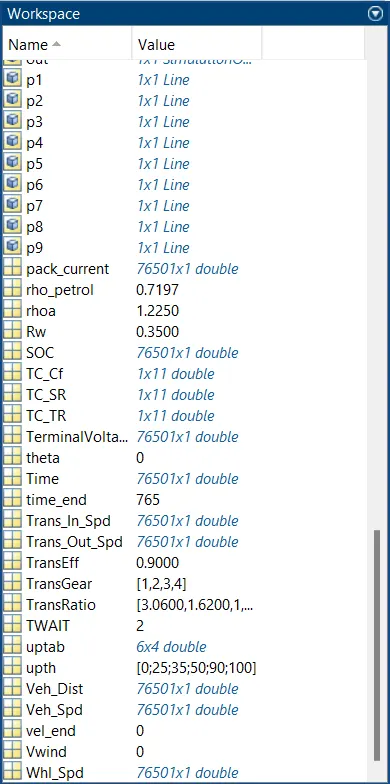
- Then the fuel economy is calculated and tabulated along with the average speed of the vehicle and displayed in the work space
- Then the plotting is done using the plot() command and countour() command.figure() command is used to plotting differernt figures and to plot multiple graphs in same figure subplot() command is used.
- Plot for time trace for engine, transmission input, transmission output and wheel speed is plotted.
- Plot for engine torque, engine power, fuel rate and fuel consumption using subplots were plotted.
- Plot for accelerator and brake pedal, gear command, vehicle desired and actual speed, vehicle distance using subplots were ploted.
- Plot for the engine operating points on the engine fuel map were ploted.
- Plot for motor speed, torque, motor input power using subplots were ploted.
- Plot for pack voltage, current and SoC using subplots were ploted.
- Plot for the motor operating points on the motor input power map, with the motor max motoring and generating torque curves were plotted.
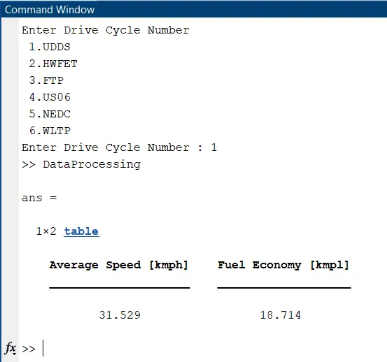
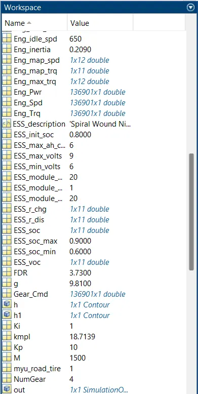
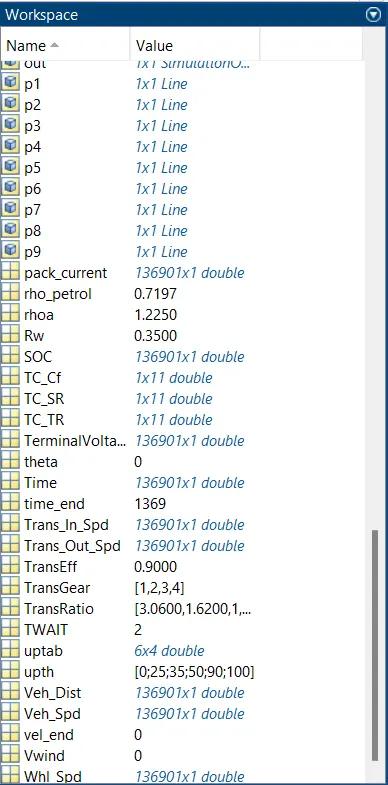
COMMANS WINDOW [UDDS]
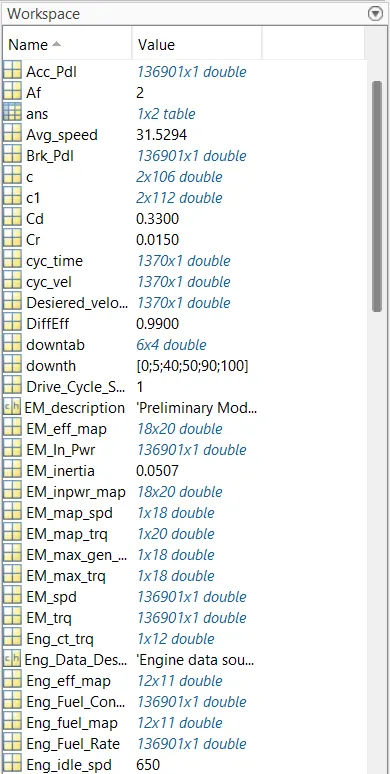
Workspace
RESULT
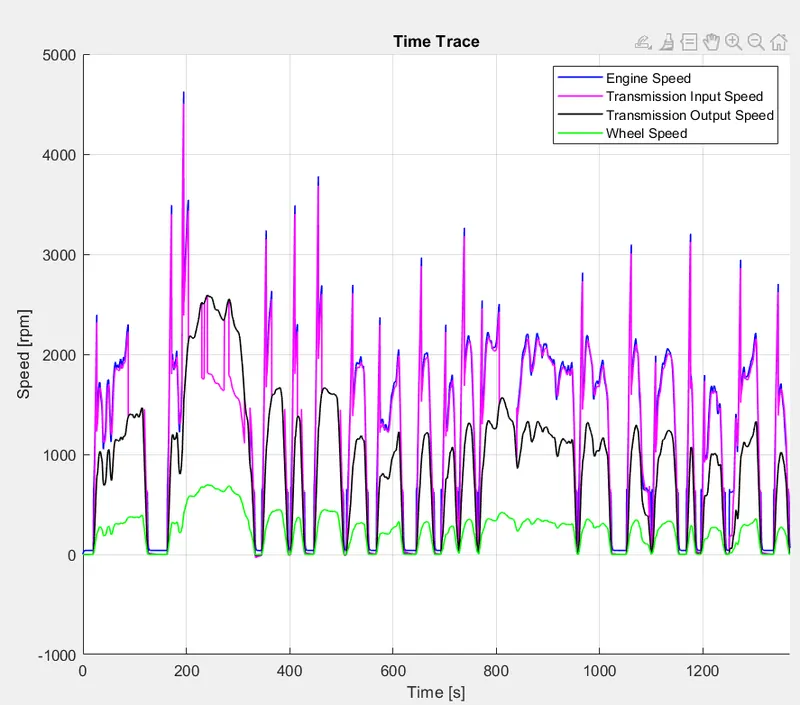
- In this all the values were highly fluctating, this is because of sudden stops, braking and acclerations.
- Also the engine speed and transmission input speed has slight variation.
Engine torque, engine power, fuel rate and fuel consumption (Engine parameters) : UDDS Drive Cycle
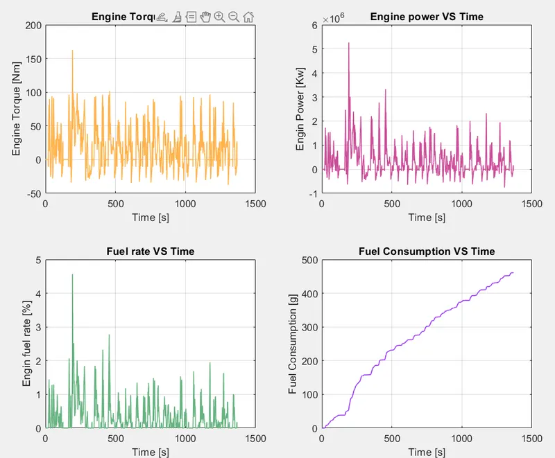
- Here the fuel consumption found to be around 461 g and the graph is also having fluctuations.
- Since it a city drive cycle all the graphs have high amount of fluctations due to sudden braking, stoping and accleration.
Accelerator and brake pedal, gear command, vehicle desired and actual speed, vehicle distance : UDDS Drive Cycle
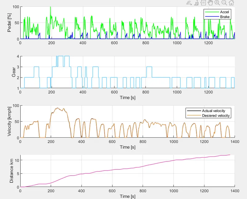
- From the graph it is clear that the brake peddal is applied frequently throughout the drive cycle.
- Also the gear is being shifted frequently between low an top.
- Lookin at the velocity graph the velocity is not at all constant at any point rather it is dropping and raising throughout the drive cycle
Engine operating points on engine fuel map : UDDS Drive Cycle
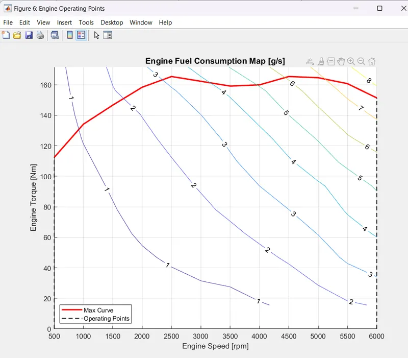
- Here we can see the maxium operating speed of the engine is between 500 rmp and 6000 rpm which is bounded by the Maximum torque curve.
UDDS Drive Cycle
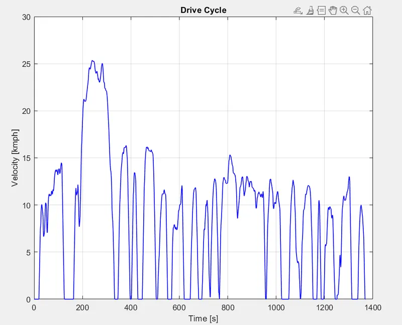
- The drive cycle reasembles the city driving the velocity of the vehicle always keeps on changing at high frequency rate.
Pack voltage, current and SoC : HWFET
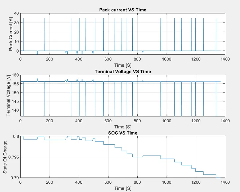
- We can see that the SOC is dropping from the initial state and regen is happening rarely.
- Also the pack current and terminal voltage bounce rapidly.
The motor operating points on the motor input power map, with the motor max motoring and generating torque curves : UDDS
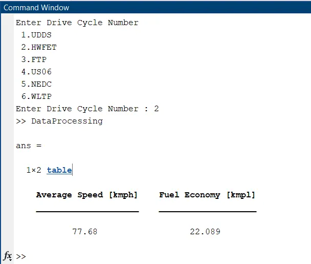
COMMAND WINDOW [HWFET]
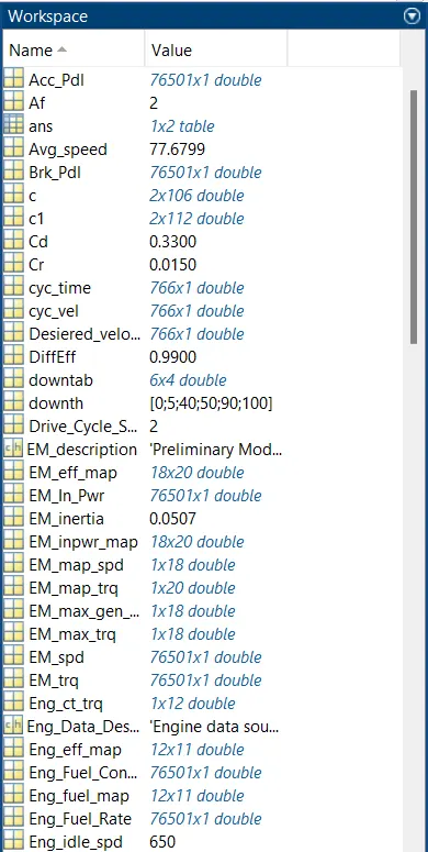
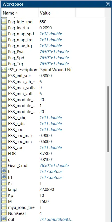
WORKSPACE
RESULT
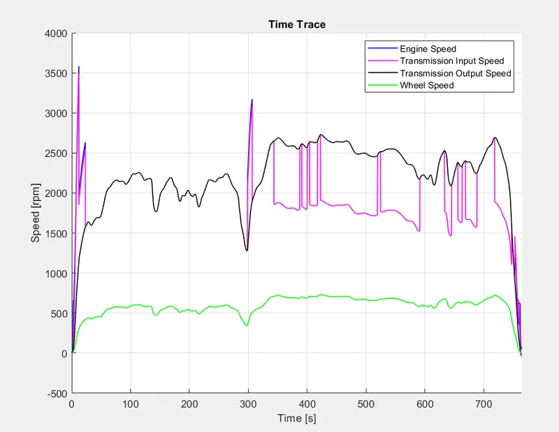
- From the graph we dont find any quick changes since it Highway drive cycle.
- The transmission input and output speed is found to be nearly consides eachother.The case of engine speed is also similar.
Engine torque, engine power, fuel rate and fuel consumption (Engine parameters) : HWFET Drive Cycle
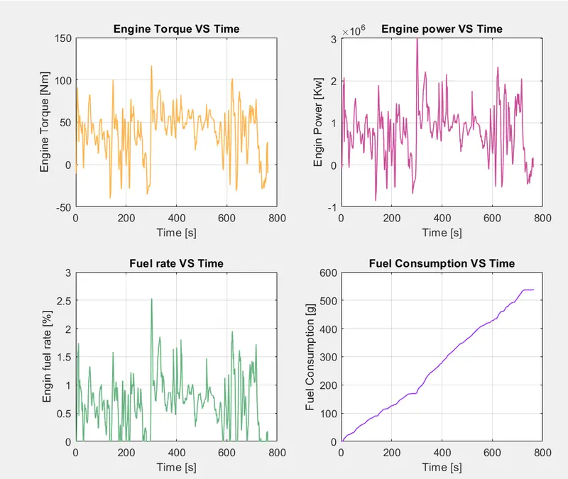
- The total fuel consumption of the entire trip is found to be around 537 g.
- Compared to UDDS the HWFET has less fluctation.
Accelerator and brake pedal, gear command, vehicle desired and actual speed, vehicle distance : HWFET Drive Cycle
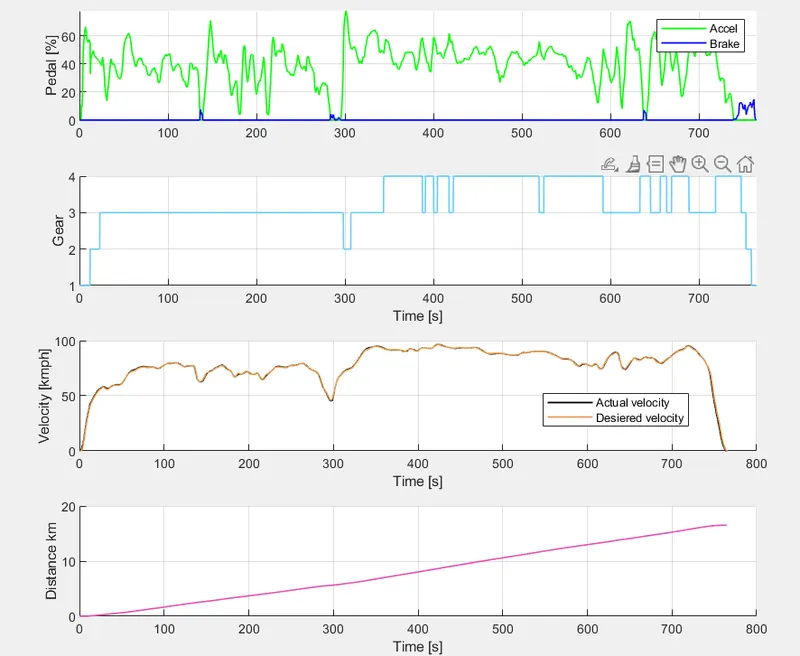
- From the graph is very clear that through out the cycle the brake peddel is applied very rarely since it is a highway driving.
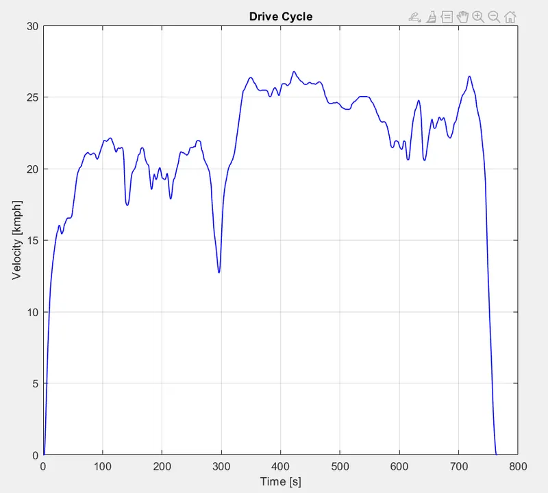
- Also by looking to the velocity graph we can find that the velocity most of the time is above 50 kmph.
Engine operating points on engine fuel map : HWFET Drive Cycle
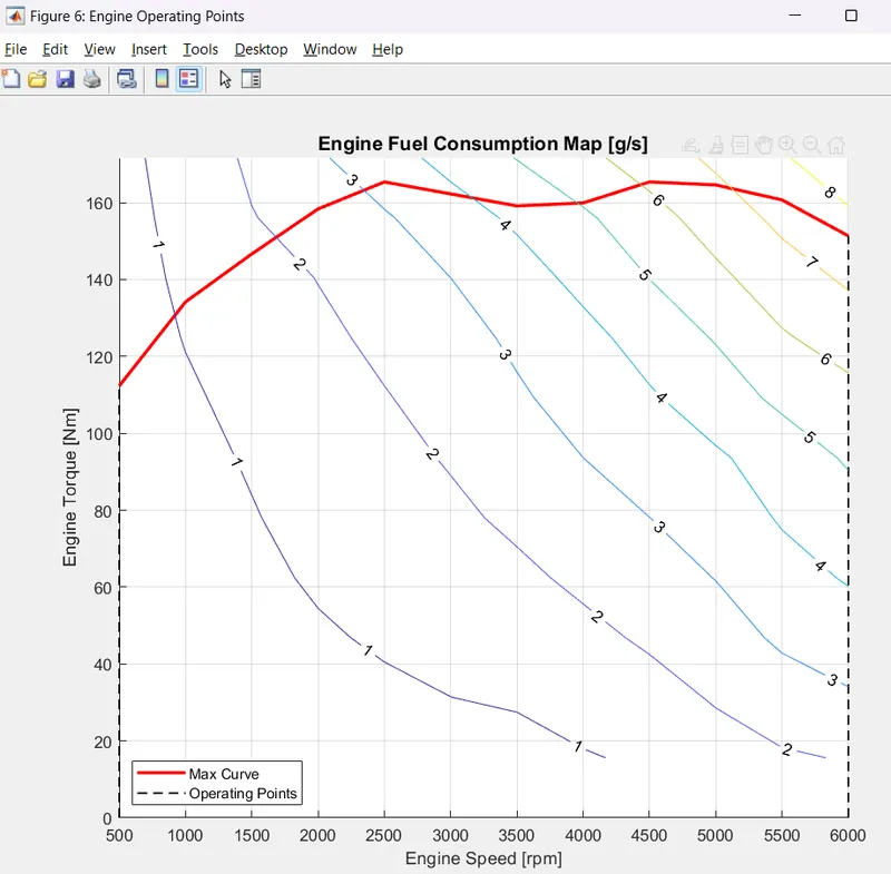
- Here we can see the maxium operating speed of the engine is between 500 rmp and 6000 rpm which is bounded by the Maximum torque curve.
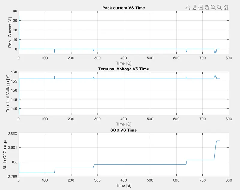
- In this scope we can find a drastic change form that we saw in UDDS deive cycle.
- In UDDS the SOC was gradually decreasing, but in HWFET the SOC went down quickly and then stated to gain charge.
- This shows that the regen is high in HWFET and the other reason is that there is very less gear shifting and braking.
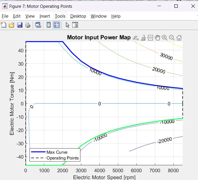
The motor operating points on the motor input power map, with the motor max motoring and generating torque curves : HWFET
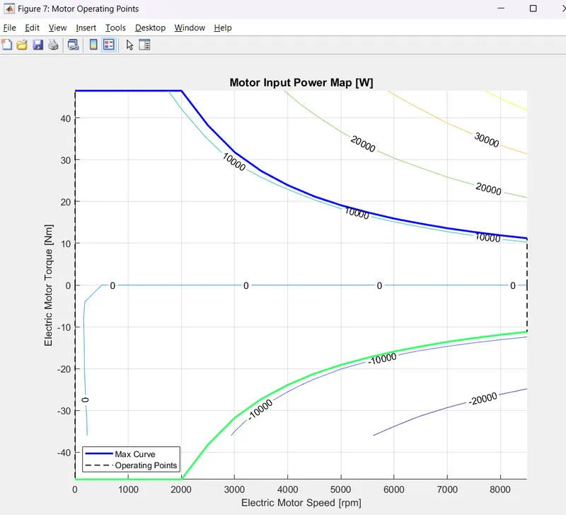
- From the graph we can find that the motor operating point is the speed between 0 rpm and 8500 rpm which is bounded by the max torque while motoring which is 46 Nm and generating torque curve which is also 46 Nm.
CONCLUSION
- The Fuel economy of UDDS Drive cycle for P1 hybrid is obtained as 18.714 kmpl where as for Conventional Vechicle it was 16.853 kmpl.
- The Fuel Economy of HWFET Drive Cycle is obtained as : 22.08 kmpl for the P1 Hybrid where as for Conventional Vechicle it was 21.20 kmpl.
- The use of Electric motor shows at the P1 state shows a raise in the fuel economy in both drive cycles.
REFERENCES
https://x-engineer.org/mild-hybrid-electric-vehicles-mhev-types/