Project 2
Aim:The task of this project is to quantify the improvement in fuel economy numbers for the hybrid vehicle (kmpl), compared to the conventional vehicle, on the urban cycle (UDDS) and highway cycle (HWFET). Also, to analyze and understand the vehicle operating points in terms of engine and motor speed, torque, transmission speeds, pedal positions, gear, distance traveled, battery voltage, current, SoC.
Theory: The transport sector has increased about 40% since 1990 but the depletion of petroleum and the increase of pollutants lead the manufacturers to develop other transportation systemsolutions. The Utopian solution would be to replace all the conventional vehicles by Electric Vehicles (EVs) but theirstorage device is limited. An intermediate solution is Hybrid
Electric Vehicles (HEVs) but these vehicles are difficult to analyze and their energy management is complex.
The purpose of this technical paper is to compare two approaches of control strategy (forward and backward)currently used to determine best practices. Since the objectiveis to compare two approaches the studied vehicle will be asimple EV represented This choice allows to be more focused on the comparison and not in the determination of hybrid supervision control, which is difficult to define. So, the work is to compare the Energetic MacroscopicRepresentation (EMR – forward approach) with WarwickPowertrain Simulation Tool for Architectures (WARPSTAR– backward approach).EMR is a graphical description exclusivelybased on physical causality (i.e. integral causality) . This property enables a straightforward deduction of a control scheme that can be implemented in real-time, that is not the case for other graphical descriptions. Such a dynamic modelling highlights energy properties of the power components such as energy storage, energy conversion and energy distribution. Moreover, an inversion-based control canbe systematically deduced from EMR, step-by-step, by
inverting the elements. WARPSTAR is a modelling package for investigation of HEVs architectures. WARPSTAR offers a full range of functionality in one structure, due to thenon-causal approach, facilitating inverse dynamic Calculations. It also has pre-built models of all knownarchitectures, and a component model library to build new .the proposed vehicle model architecture improves modelling flexibility by standardizing and replicating the real physical coupling between model subsystems. This allows for rapid reconfiguration of the model as well as testing and validation of individual component subsystems in isolation. The addition of an external torque source represented the addition of a hybridizing component to the drivetrain. Due to the new VMA, the external torque source was easily incorporated without excessive modification to the existing drivetrain. It has been shown that the proposed modelling methodology is suitable for the simulation of vehicle dynamics closely matching real world driving data. The new VMA can also include complex components such as clutches and torque convertors, accurately accounting for coupling and decoupling within the powertrain system. The use of the Simulink environment rather than a commercial package also benefits the user/developer by giving extra freedom in model development that other commercial packages may not give. Further work is to be completed on full drive cycle analysis using the new flexible architecture. Full validation of the model will also be performed to both conventional and hybrid drivetrain configurations. Development will also be conducted on the hybrid component models such as motor generator units and energy storage systems to improve the accuracy of the input data to the model whilst allowing additional results to be extracted.
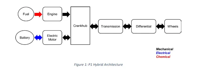
P1 Mild Hybrid Electric Vehicle:-
The P1 architecture, with the electric machine connected directly to the crankshaft, is the solution adopted by Honda on their first generation Integrated Motor Assist (IMA) technology. The electric motor functions as a generator, during vehicle deceleration, as an engine starter, and as a motor (to assist the engine) during vehicle accelerations. One of the biggest advantage of this solution is that the electric motor can provide higher torque than the BiSG, since there is no belt limitation (due to slip). However, since there is no speed / torque ratio between the electric machine and crankshaft, the torque requirements on the electric motor can be quite demanding.
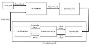
In this model We use Forward Model:-
`t also known as dynamic simulation. Dynamic models are used for detailed simulations. In this model force/torque/power is the input and the vehicle state variable velocity and acceleration are outputs. The models and simulatios are more realistic due to phhysical casualty hence appropriate for control development. There is feedback loop to meet the desired vehicle state. It is mainly used to simulate a vehicle on a driving cycle to analyse the dynamic behaviour of the system helps significantly in control development`
%% Skill-Lync -> Hybrid Drives Development
% Project 2 - P1 Hybrid Vehicle Model
% By - Gunashekar
% Description:
%% Initialization File
% Initialization file for loading the variables for the Conventional vehicle simulation model
%% Vehicle Parameters
M = 1500; % Vehicle weight [kg]
Cr = 0.015; % Rolling resistance coefficient
Rw = 0.35; % Rolling radius [m]
Cd = 0.33; % Drag coefficient
Af = 2; % Frontal area [m2]
rhoa = 1.225; % Air density [kg/m3]
Vwind = 0; % Wind velocity [kmph]
g = 9.81; % Gravitational acceleration [m/s2]
theta = 0; % Slope [deg]
myu_road_tire = 1; % Coefficient of friction between tire - road interface
%% Powertrain Parameters
FDR = 3.73; % Final Drive Ratio / Diff Ratio
DiffEff = 0.99; % Differential efficiency (assumed independent of operating conditions)
NumGear = 4; % Number of gears in transmission
TransGear = [1:NumGear]; % Transmission Gears
TransRatio = [3.06, 1.62, 1, 0.7]; % Corresponding Transmission ratios
TransEff = 0.90; % Transmission efficiency (assumed independent of operating conditions)
TC_SR = [0, .5, .6, .7, .8, .87, .92, .94, .96, .97, 1]; % Torque Converter Speed Ratio (Matlab default) -> TurbSpd/PumpSpd
TC_TR = [2.232, 1.5462, 1.4058, 1.2746, 1.1528, 1.0732, 1.0192, 1, 1, 1, 1]; % Torque Converter Torque Ratio (Matlab default) -> TurbTrq/PumpTrq
TC_Cf = 1e-4 * [.72558, .66322, .63463, .59042, .51331, .4144, .29287, .22444, .12186, .04386, 0]; % Torque Converter Capacity Factor (Matlab default) -> PumpTrq/PumpSpd^2 [Nm/rpm^2]
load Engine_data_1_9L_Saturn_95kW
load Trans_Shift_map
load EM_Honda_Insight_10kW
load ESS_NiMH6
ESS_init_soc = 0.8;
ESS_soc_max = 0.9;
ESS_soc_min = 0.6;
Eng_idle_spd = 600;
SOC_max = 0.9;
SOC_min = 0.6;
%% Driver Parameters
Kp = 10; % P gain for driver PI model
Ki = 1; % I gain for driver PI model
Drive_Cycle_Select = 1; % Drive cycle selection
% Drive cycle values in m/s
if Drive_Cycle_Select == 1
load DriveCycles/UDDS;
elseif Drive_Cycle_Select == 2
load DriveCycles/HWFET;
elseif Drive_Cycle_Select == 3
load DriveCycles/FTP;
elseif Drive_Cycle_Select == 4
load DriveCycles/US06;
elseif Drive_Cycle_Select == 5
load DriveCycles/NEDC;
elseif Drive_Cycle_Select == 6
load DriveCycles/WLTP;
end
time_end = cyc_time(end);
vel_end = cyc_vel(end);
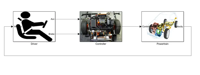
Simulink Model :
Driver:
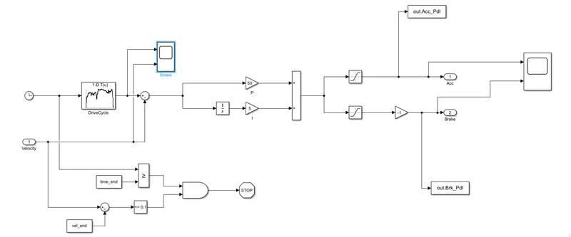
It is modeled using a ‘Driver’ block, which is a basic PI controller that generates accelerator and brake pedal outputs to match the desired and actual vehicle speeds.
Controller:
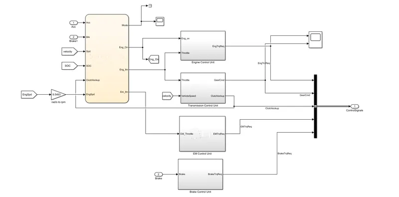
The Controller block is the brains of the vehicle, representing the electronic controls units. It is based on the driver inputs, it generates desired engine torque, desired transmission gear desired motor torque and desired brake torque. These inputs are fed to the ‘Powertrain’ block which represents the drivetrain of the vehicle
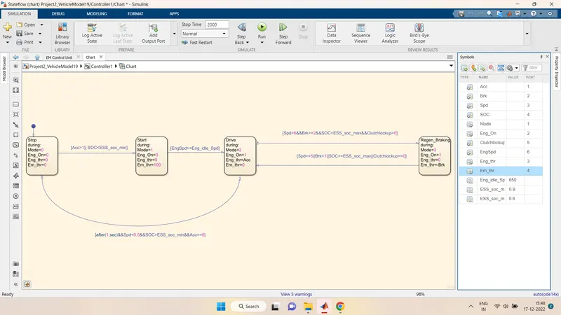
Stateflow for Controller:
Engine Control Unit:
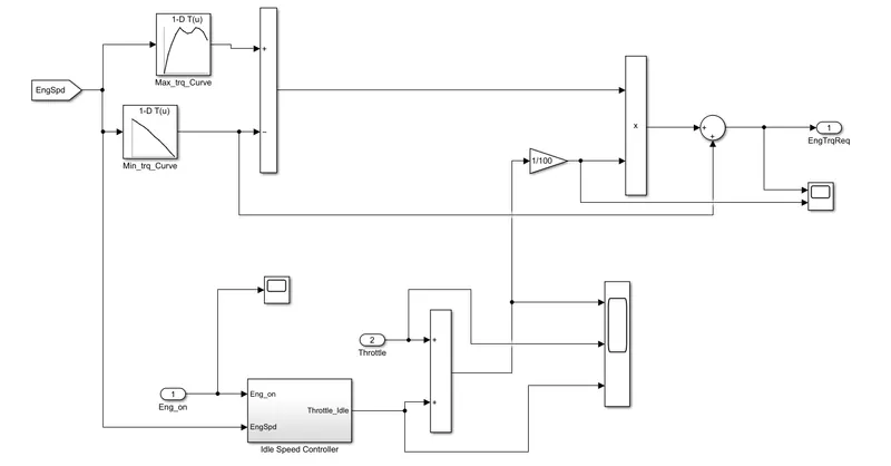
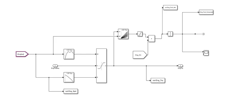
In this control model We use engine control unit in that give input Engine speed through creating look up table. in that table we give input Maximum torque and map speed then also create 2nd look up trable in that give input ct torque and map speed then it substracts and multiplied. the engine speed also give to ideal contro speed to integrate from this we meet output of engine required torque
Transmission Control Unit:
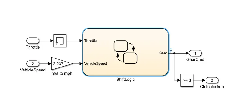
Shiftlogic In this unit:
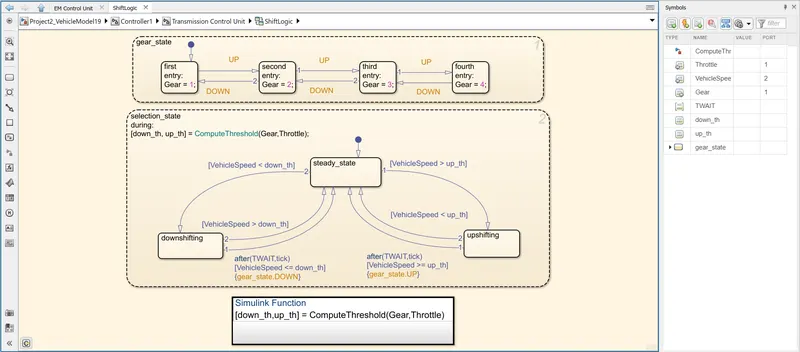
In this unit we create steadfy flow variable state for controlling of gears of vehicle as in ascending and descending order with respect to time, speed, distance. and give input to this steady state is vehicle speed in m/s to mph
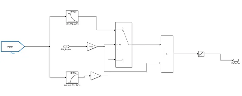
Electric Motor Control Unit
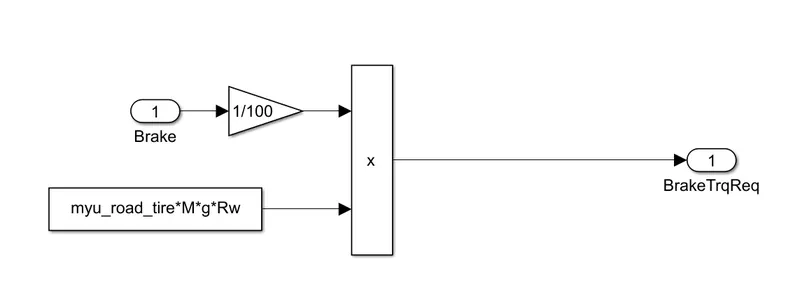
Brake Control Unit:
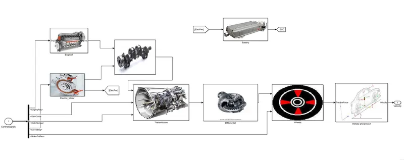
Powertrain:
A powertrain is an assembly of every component that thrusts your car into motion. It includes engine, transmission, driveshaft, axles, and differential
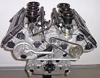
Engine:
Electric Motor:
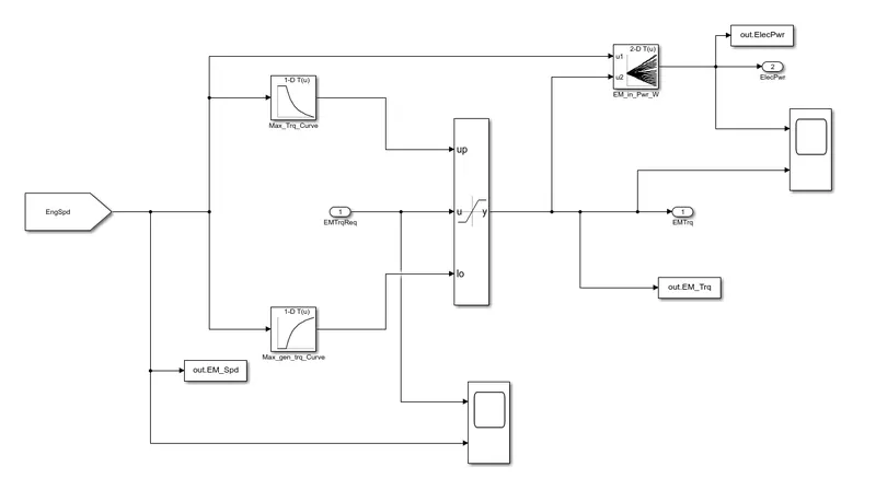
An electric motor is an electrical machine that converts electrical energy into mechanical energy. Most electric motors operate through the interaction between the motor's magnetic field and electric current in a wire winding to generate force in the form of torque applied on the motor's shaft
Crankhub:
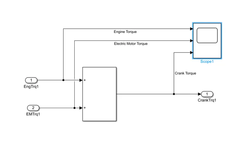
The Stock Crank Hub design allows the timing gear to spin independently from the crank causing the user to get the engine re-timed at a minimum and in worst case scenario cause piston to valve contact damaging the engine and requiring a complete engine overhaul.
Transmission:
Propulsion transmission is the mode of transmitting and controlling propulsion power of a machine. The term transmission properly refers to the whole drivetrain, including clutch gearbox, prop shaft (for rear-wheel drive vehicles, and final drive shafts.
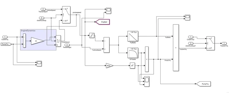
Torque Converter:
The torque converter is what transmits that torque from the engine to a rotating driven load. In an automatic transmission car, the torque converter connects the power source to the load. Torque converters are comprised of five main components: the impeller, the turbine, the stator, a clutch, and the fluid
Differential:
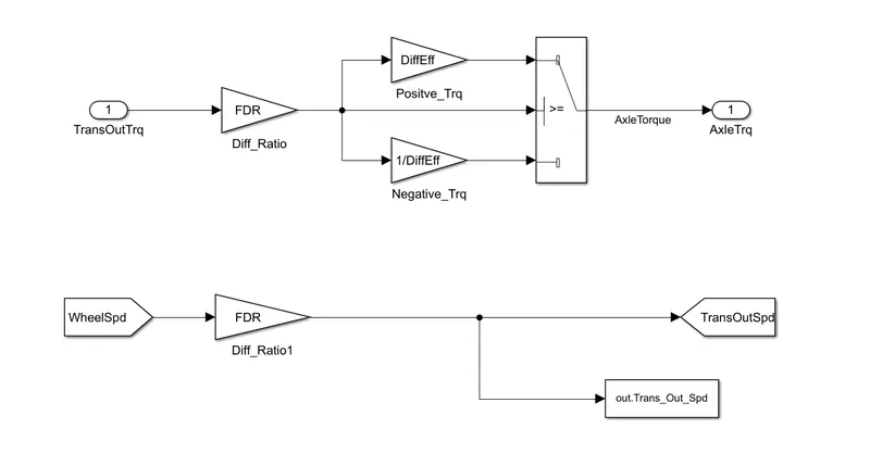
A differential is a gear train with three drive shafts that has the property that the rotational speed of one shaft is the average of the speeds of the others, or a fixed multiple of that average
Wheel:
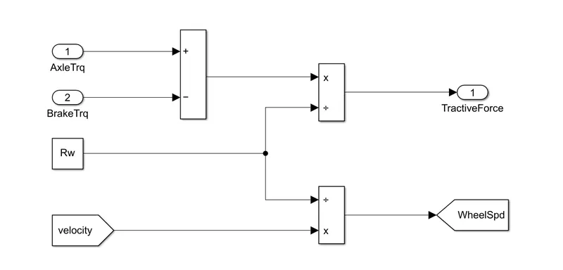
Vehicle Dynamics:
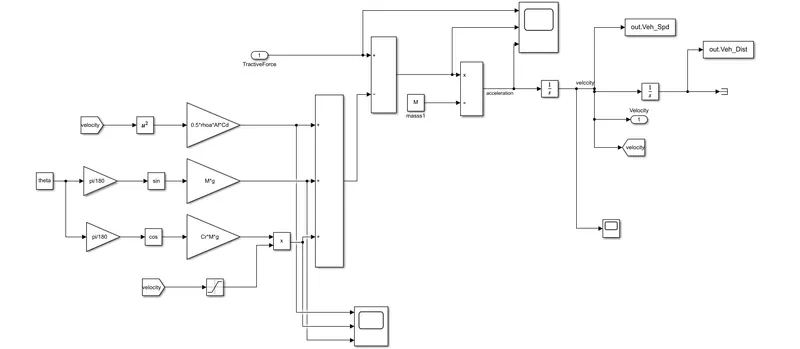
For motorized vehicles, such as automobiles, aircraft, and watercraft, vehicle dynamics is the study of vehicle motion, e.g., how a vehicle's forward movement changes in response to driver inputs, propulsion system outputs, ambient conditions, air/surface/water conditions
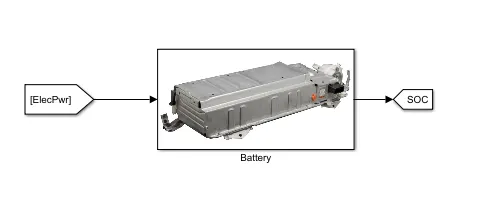
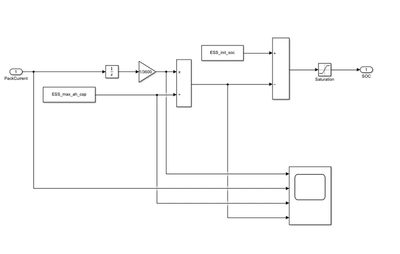
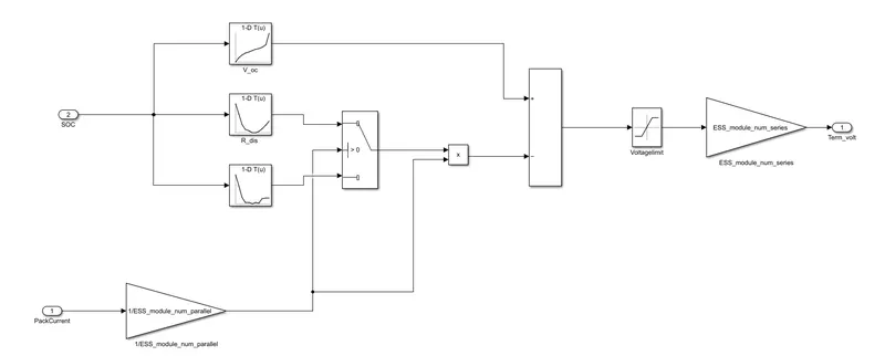
Battery Modeling :
Post process :
%% Renaming variables
Time = out.tout;
Acc_Pdl = out.Acc_Pdl; % Accelerator pedal [%]
Brk_Pdl = out.Brk_Pdl; % Brake pedal [%]
Gear_Cmd = out.Gear_CMD; % Transmission gear
Trans_In_Spd = out.Trans_In_Spd*30/pi; % Transmission input speed [rpm]
Trans_Out_Spd = out.TransOutSpd*30/pi;% Transmission output speed [rpm]
Eng_Trq = out.Eng_Trq; % Engine brake torque [Nm]
EngSpd = out.EngSpd*30/pi; % Engine speed [rpm]
Eng_Fuel_Consump = out.Eng_Fuel_Consumption; % Engine fuel consumption [g]
Veh_Dist = out.Veh_Dist/1000; % Distance traveled by vehicle [km]
Veh_Spd = out.Veh_Spd*18/5; % Vehicle speed [kmph]
Wheel_Speed = out.WheelSpeed; % Wheel speed [kmph]
Eng_Fuel_Rate = out.Eng_Fuel_Rate; % Engine fuel rate [%]
EM_Speed = out.EMSpd*18/5; % Electric Motor Speed
EM_Power = out.EMPwr; % Electric Motor Power
EM_Torque = out.EMTrq; % Electric Motor Torque
Term_Volt = out.term_volt; % Terminal Voltage of battery
Soc = out.SOC; % State Of Charge
Pack_Current = out.Pack_Current; %Pack current of battery
%% Data Analysis
Eng_Pwr = Eng_Spd*pi/30*Eng_Trq/1000; % Engine brake power [kW]
rho_petrol = 0.7197; % Density of petrol [kg/L]
kmpl = Veh_Dist(end)/(Eng_Fuel_Consump(end)/1000/rho_petrol); % Fuel economy [kmpl]
%% Plotting vehicle characteristics time trace to Engine speed, Engine Torque, Engine Power,
% And Engine fuel rate, Engine fuel consumption
% Data conversion from Double Timeseries
Eng_Spd = Eng_Spd.Data(:,1); % engine speed
Eng_trq = Eng_Trq.Data(:,1); % engine torque
Eng_pwr = Eng_Pwr.Data(:,1); % engine power
Eng_fuel_rate = Eng_Fuel_Rate.Data(:,1); % engine fuel rate
Eng_fuel_consumption = Eng_Fuel_Consump.Data(:,1); % engine fuel consumption
EM_speed = EM_Speed.Data(:,1); % motor speed
EM_power = EM_Power.Data(:,1); % Motor Power
EM_torque = EM_Torque.Data(:,1); % Motor Torque
Pack_current = Pack_Current.Data(:,1); %pack current of battery
State_of_charge = Soc.Data(:,1); %state of charge
Term_voltage = Term_Volt.Data(:,1); % terminal Voltage of battery
%% Plotting vehicle characteristics time trace transmission IN/OUT and Wheel Speed
figure(1)
hold on
grid on
plot(Time, Trans_In_Spd, 'linewidth', 1, 'Color', 'black');
plot(Time, Trans_Out_Spd, 'linewidth', 1, 'Color', 'red');
plot(Time, Wheel_Speed, 'linewidth',1, 'color', 'blue')
ylabel('Speed [rpm]')
xlabel('Timem [s]')
xlim([0, Time(end)]);
ylim([0, 6000]);
legend('Trans Input','Trans Output','Wheel Speed');
%% Plotting Engine speed, Engine Torque, Engine Power,Engine fuel rate,Engine fuel consumption wrt Time
figure(2)
subplot(4,1,1)
plot(Time,Eng_trq,'linewidth',1,'color','black')
xlim([0, Time(end)]);
xlabel('Time [s]')
ylabel('Torque [Nm]')
legend('Engine Torque')
grid on
subplot(4,1,2)
plot(Time,Eng_pwr,'linewidth',1,'color','blue')
xlim([0, Time(end)]);
xlabel('Time [s]')
ylabel('Power [KW]')
legend('Engine Power')
grid on
subplot(4,1,3)
plot(Time,Eng_fuel_rate,'linewidth',1,'color','red')
xlim([0, Time(end)]);
xlabel('Time [s]')
ylabel('Fuel Rate [%]')
legend('Engine Fuel Rate')
grid on
subplot(4,1,4)
plot(Time,Eng_fuel_consumption,'linewidth',1,'color','green')
xlim([0, Time(end)]);
xlabel('Time [s]')
ylabel('Fuel Consumption')
legend('Engine Fuel Consumption')
grid on
% Plotting fuel economy Vs Engine Fuel consumption
figure(3)
plot(Eng_fuel_consumption,Eng_fuel_rate,'color','r')
xlabel('Fuel consumption')
ylabel('Fuel Rate [%]')
title('Fuel economy Vs Fuel Consumption')
grid on
%% Potting Accelerator pedal, Brake pedal and gear command with respect to time
figure(4)
subplot(2,1,1)
hold on
plot(Time, Acc_Pdl, 'linewidth', 1, 'Color', 'black');
plot(Time, Brk_Pdl, 'linewidth', 1, 'Color', 'red');
ylabel('Pedal [%]')
xlabel('Time [s]');
xlim([0, Time(end)]);
grid on
legend('Accel','Brake');
title('Acceleration & Brake Pedal wrt Time')
subplot(2,1,2)
plot(Time, Gear_Cmd, 'linewidth', 1, 'Color', 'black');
xlim([0, Time(end)]);
xlabel('Time [s]');
ylabel('Gear');
grid on
title('Gear command wrt Time')
% Plotting gear command vehicle desired with actual speed
figure(5)
subplot(2,1,1)
plot(Veh_spd, Gear_Cmd, 'linewidth', 1, 'Color', 'black');
xlabel('Speed [rpm]');
ylabel('Gear');
grid on
title('Gear command wrt vehicle speed')
subplot(2,1,2)
plot(Veh_dist, Gear_Cmd, 'linewidth', 1, 'Color', 'red');
xlabel('Distance [kmpl]');
ylabel('Gear');
grid on
title('Gear command wrt Distance')
%% Plotting engine operating points on engine fuel map
figure('Name','Engine Operating Points');
hold on
grid on
title('Engine Operating Points','fontsize',12);
p1=plot(Eng_map_spd*30/pi,Eng_max_trq,'linewidth',2,'color','r');
p2=line([Eng_map_spd(end)*30/pi Eng_map_spd(end)*30/pi],[0 Eng_max_trq(end)]);
set(p2,'linewidth',1,'linestyle','--','color','k');
p3=line([Eng_map_spd(1)*30/pi Eng_map_spd(1)*30/pi],[0 Eng_max_trq(1)]);
set(p3,'linewidth',1,'linestyle','--','color','k');
[c,h] = contour(Eng_map_spd'*30/pi,Eng_map_trq,Eng_fuel_map');
clabel(c,h);
xlabel('Engine Speed [rpm]');
ylabel('Engine Torque [Nm]');
title('Engine Fuel Consumption Map [g/s]');
legend([p1 p3],{'Max Curve','Operating Points'});
axis([Eng_map_spd(1)*30/pi Eng_map_spd(end)*30/pi 0 Eng_map_trq(end)]);
%% State of Charge, Pack Current, And Terminal Voltage with respect to Time
figure(6)
subplot(3,1,1)
plot(Time,Pack_current,'linewidth',1,'color','black')
xlim([0, Time(end)]);
xlabel('Time [s]')
ylabel('Current [W]')
legend('Pack Current')
grid on
subplot(3,1,2)
plot(Time,State_of_charge,'linewidth',1,'color','blue')
xlim([0, Time(end)]);
xlabel('Time [s]')
ylabel('Charging [%]')
legend('State Of Charge')
grid on
subplot(3,1,3)
plot(Time,Term_voltage,'linewidth',1,'color','red')
xlim([0, Time(end)]);
xlabel('Time [s]')
ylabel('Voltage [V]')
legend('Terminal Voltage')
grid on
%% Motor Speed, Torque, Motor input power with respect to Time
figure(7)
subplot(3,1,1)
plot(Time,EM_power,'linewidth',1,'color','black')
xlim([0, Time(end)]);
xlabel('Time [s]')
ylabel('Power [W]')
legend('Electric Motor Power ')
grid on
subplot(3,1,2)
plot(Time,EM_torque,'linewidth',1,'color','blue')
xlim([0, Time(end)]);
xlabel('Time [s]')
ylabel(' Torque [Nm]')
legend('Electric Motor Torque')
grid on
subplot(3,1,3)
plot(Time,EM_speed,'linewidth',1,'color','red')
xlim([0, Time(end)]);
xlabel('Time [s]')
ylabel('Speed [Rpm]')
legend('Electrical Motor Speed')
grid on
%% Plotting EM Operating Points on motor input power Map
figure('Name','Electric Motor Operating Points');
hold on
grid on
title('Electric Motor Operating Points','fontsize',12);
p1=plot(EM_map_spd*30/pi,EM_max_trq,'linewidth',2,'color','r');
p2=line([EM_map_spd(end)*30/pi EM_map_spd(end)*30/pi],[0 EM_max_trq(end)]);
set(p2,'linewidth',1,'linestyle','--','color','k');
p3=line([EM_map_spd(1)*30/pi EM_map_spd(1)*30/pi],[0 EM_max_trq(1)]);
set(p3,'linewidth',1,'linestyle','--','color','k');
[c,h] = contour(EM_map_spd'*30/pi,EM_map_trq,EM_inpwr_map');
clabel(c,h);
xlabel('Motor Speed [rpm]');
ylabel('Motor Torque [Nm]');
title('Motor Input Power Map [g/s]');
legend([p1 p3],{'Max Curve','Operating Points'});
axis([EM_map_spd(1)*30/pi EM_map_spd(end)*30/pi 0 EM_map_trq(end)]);
Result:
Fuel Economy Numbers for project 2
| S.No | Drive cycle | Fuel Economy Number (KMpl) |
| 1 | UDDS | 19.22 |
| 2 | HWFET | 17.1613 |
As we see the fuel economy is high in HWFET compared to UDDS. It is because in urban driving the vehicle encounters more traffic and it has to stop for fever distance and it consumes more fuel at the starting. In HWFET the vehicle encounters no traffic and it moves without use of too much braking so it will have more fuel economy number.
Plot for USSD and HWFET derive Cycle:
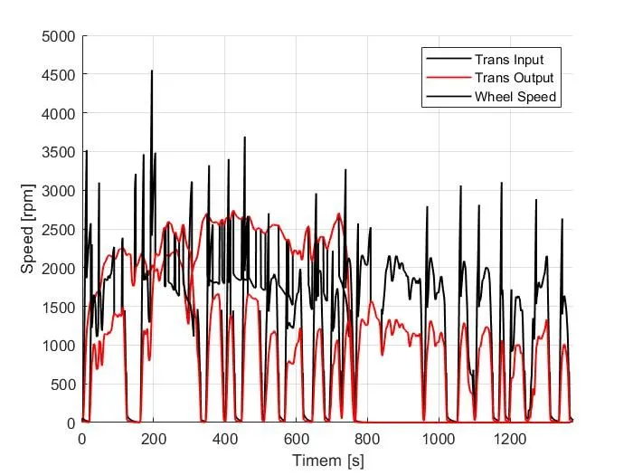
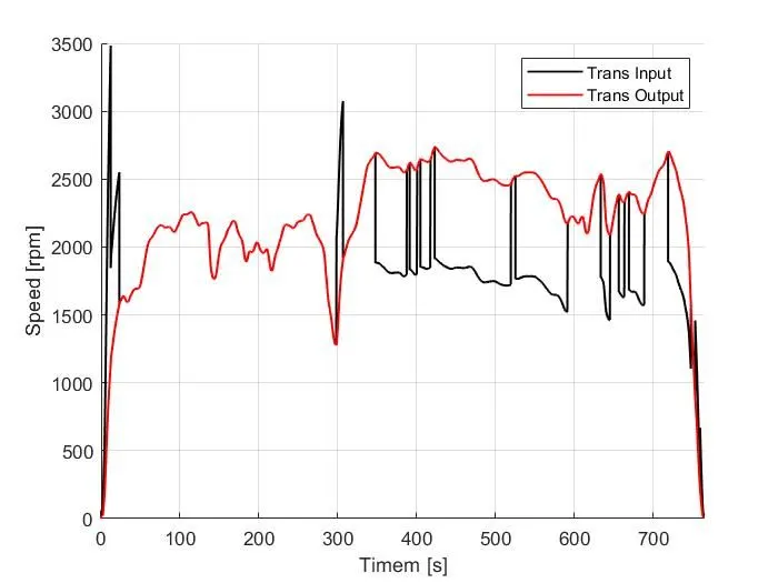
1. Plotting the vehicle characteristic Time Trace, Transmission of IN/OUT and Wheel Speed
For USSD drive Cycle:
For HWFET drive Cycle:
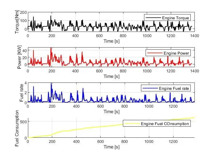
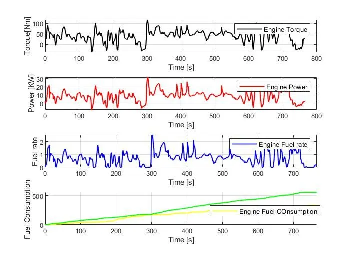
2. Potting the vehicle characteristic Time trace to Engine Torque ,Engine Power,Engine fuel rate and Engine fuel consumption
For HWFET drive Cycle:
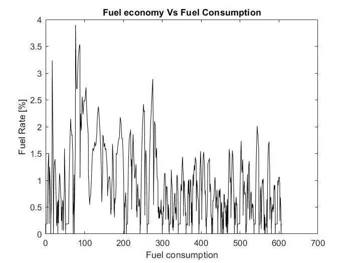
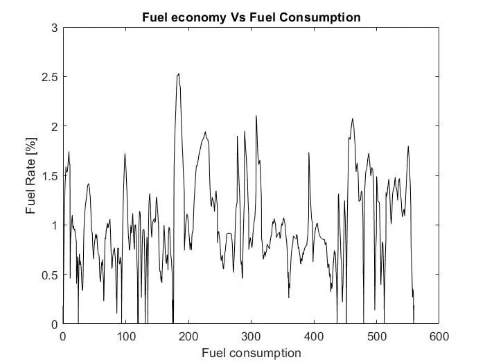
3.Plotting of Fuel Economy vs Fuel Consumption
For USSD drive Cycle:
For HWFET drive Cycle:
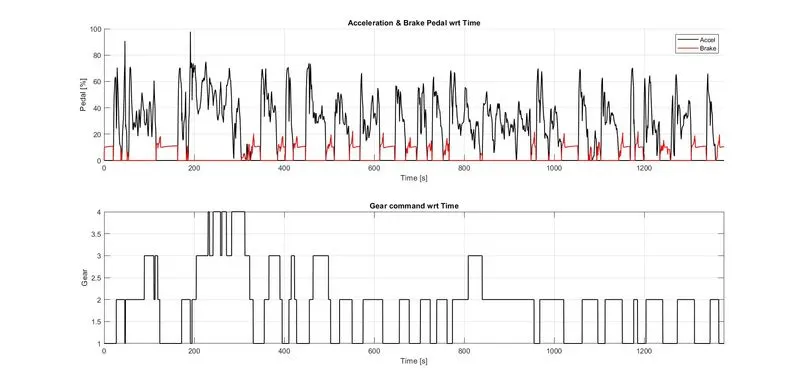
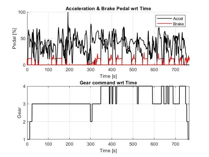
4.Plotting the Accelaration pedal,break pedal and gear command with respect to time
For USSD drive Cycle:
For HWFET drive Cycle:
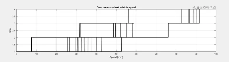
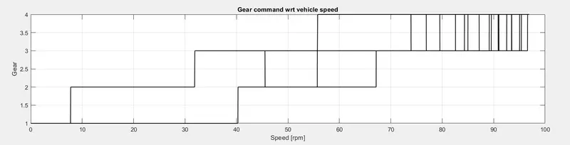
5.Plotting Gear command with Vehicle speed and distance:
For USSD drive Cycle:
For HWFET drive Cycle:
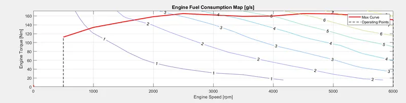
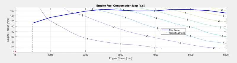
PLotting the Engine fuel consumption map:
For USSD drive Cycle:
For HWFET drive Cycle:
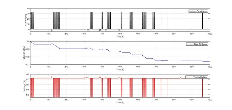
lot pack voltage, current and SoC using subplot
For UDDS drive cycle:-
For HWFET drive cycle:
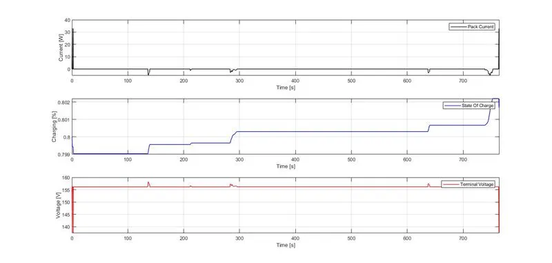
The pack voltage and current will have more fluctuations in UDDS as compared to HWFET cycle because of the frequent start and stops throughout the drive and the battery has to provide the energgy everytime when the car is starting from the idle position.SOC decreased in the UDDS cycle wrt time but it has increased in HWFET cycle. It is because in UDDS we have frequent start and stops and battery has to provide the energy has evertytime when the caris starting from the idle position and the SOC decreases but in HWFET cycle The Vehicle will be moving continuously without braking frequently and the alternator is utilised to transfer some engine power to the battery through motor so SOC increase in the HWFET cycle.
Plot the motor operating points on the motor input power map, with the motor max motoring and generating torque curves:
For UDDS drive cycle:
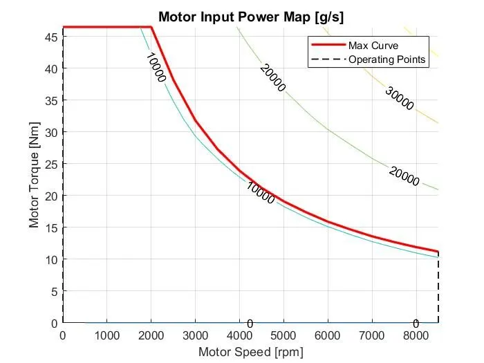
For HWFET drive cycle:
The various performance of characteristics and operating points of UDDS drive cycle and HWFET drive cycle are analysed and the graphs are plotted
- Time trace for engine, Transmission input, Transmission output and wheelspeed with respect to time.
- Engine torque, Engine power, Fuel rate and Fuel consumption with respect to time.
- Accelerator and brake pedal, gear command and vehicle desired, actual speed, vehicle distance with respect to time.
- Engine operating points on the engine fuel map with respect to time.
- Motor speed, Torque, Motor input power with respect to time.