Week 4.1 - Genetic Algorithm
Aim :To calculate the global maixma of a stalagmite function using matlab
Theroy : The global maxima of a "stalagmite function" can be obtained using "genetic algorith" in matlab.
Introduction
The genetic algorithm (GA), developed by John Holland and his collaborators in the 1960s and 1970s (Holland, 1975; De Jong, 1975), is a model or abstraction of biological evolution based on Charles Darwin's theory of natural selection. Holland was probably the first to use the crossover and recombination, mutation, and selection in the study of adaptive and artificial systems. These genetic operators form the essential part of the genetic algorithm as a problem-solving strategy. Since then, many variants of genetic algorithms have been developed and applied to a wide range of optimization problems, from graph coloring to pattern recognition, from discrete systems (such as the travelling salesman problem) to continuous systems (e.g., the efficient design of airfoil in aerospace engineering), and from financial markets to multi-objective engineering optimization.
There are many advantages of genetic algorithms over traditional optimization algorithms. Two most notable are: the ability of dealing with complex problems and parallelism. Genetic algorithms can deal with various types of optimization, whether the objective (fitness) function is stationary or non-stationary (change with time), linear or nonlinear, continuous or discontinuous, or with random noise. Because multiple offsprings in a population act like independent agents, the population (or any subgroup) can explore the search space in many directions simultaneously. This feature makes it ideal to parallelize the algorithms for implementation. Different parameters and even different groups of encoded strings can be manipulated at the same time.
what is genetic algorithm
The genetic algorithm is a method for solving both constrained and unconstrained optimization problems that is based on natural selection, the process that drives biological evolution. The genetic algorithm repeatedly modifies a population of individual solutions. At each step, the genetic algorithm selects individuals at random from the current population to be parents and uses them to produce the children for the next generation. Over successive generations, the population "evolves" toward an optimal solution. You can apply the genetic algorithm to solve a variety of optimization problems that are not well suited for standard optimization algorithms, including problems in which the objective function is discontinuous, nondifferentiable, stochastic, or highly nonlinear. The genetic algorithm can address problems of mixed integer programming, where some components are restricted to be integer-valued.
The genetic algorithm uses three main types of rules at each step to create the next generation from the current population:
-
Selection rules select the individuals, called parents, that contribute to the population at the next generation.
-
Crossover rules combine two parents to form children for the next generation.
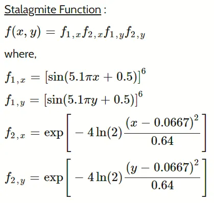
Equation used: Stalagmite function
objective :
- To optimize the stalagmite function
- To determine the global maxima of the function
Stalagmite function program
function [f] = stalagmite(input_vector)
x = input_vector(1);
y = input_vector(2);
f1 = (sin(5.1.*pi.*x+0.5)).^6;
f2 = (sin(5.1.*pi.*y+0.5)).^6;
f3 = exp((-4.*log(2).*(x-0.0667).^2)/(0.64));
f4 = exp((-4.*log(2).*(y-0.0667).^2)/(0.64));
f = -f1.*f2.*f3.*f4;
end
Main function code
clear all
close all
clc
x = linspace(0,0.6,150);
y = linspace(0,0.6,150);
num_cases = 50;
%creatind 2d mesh
[xx,yy]=meshgrid(x,y);
%calling the function
for i = 1:length(x)
for j = 1:length(y)
input_vector(1) = xx(i,j);
input_vector(2) = yy(i,j);
f(i,j)= get_stalagmite(input_vector);
end
end
%study 1 behaviour
tic
for i = 1:num_cases
[inputs1,fopt1(i)] = ga(@get_stalagmite,2);
xopt(i) = inputs1(1);
yopt(i) = inputs1(2);
end
%study time 1 =toc
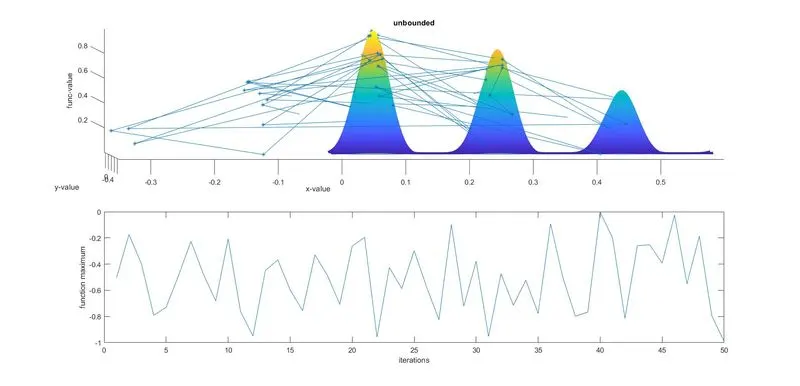
%unbounded inputs
figure(1)
subplot(2,1,1)
hold on
surfc(xx,yy,-f)
xlabel('x-value')
ylabel('y-value')
zlabel('func-value')
shading interp
plot3(xopt,yopt,-fopt1,'marker','*','markersize',5)
title('unbounded')
subplot(2,1,2)
plot(fopt1)
xlabel('iterations')
ylabel('function maximum')
%study 2 behaviour
tic
for i = 1:num_cases
[inputs,fopt(i)] = ga(@get_stalagmite,2,[],[],[],[],[0;0],[0.5;0.5]);
xopt(i) = inputs(1);
yopt(i) = inputs(2);
end
%study time 2 =toc
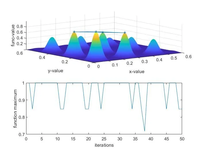
%bounded inputs
figure(2)
subplot(2,1,1)
surfc(xx,yy,-f)
xlabel('x-value')
ylabel('y-value')
zlabel('func-value')
hold on
shading interp
plot3(xopt,yopt,-fopt ,'marker','*','markersize',5)
subplot(2,1,2)
title('bounded')
plot(-fopt)
xlabel('iterations')
ylabel('function maximum')
%study increasing ga population size
options = optimoptions('ga');
options = optimoptions(options,'populationsize',200);
tic
for i= 1:num_cases
[inputs3,fopt3(i)] = ga(@get_stalagmite,2,[],[],[],[],[0;0],[1;1],[],[],options);
xopt(i) = inputs3(1);
yopt(i) = inputs3(2);
end
%study time 3 =toc
%bounded inputs
figure(3)
subplot(2,1,1)
surfc(xx,yy,-f)
xlabel('x-value')
ylabel('y-value')
zlabel('func-value')
hold on
shading interp
plot3(xopt,yopt,-fopt,'marker','o','markersize',5,'markerfacecolor','r')
subplot(2,1,2)
plot(-fopt)
title('bounded inputs increases population size687')
xlabel('iterations')
ylabel('function maximum')
Steps carried out program :
- Initial the stalagmite function was mention with appropriate arguments vectors
- the problem has been subdivided into three studies based on the limitation of preveious study
- first study deal with unbounded inputs,thereby expanding the boundary wherein the result can be obtained
- second study bring inthe aspect of bounded inputs providing a better solution for the drawback faced
- plot of all the three studies have been displayed ,thus giving a clear insight of the result
Results:
study 1 behaviour
study 2 behaviour
study 3 behaviour
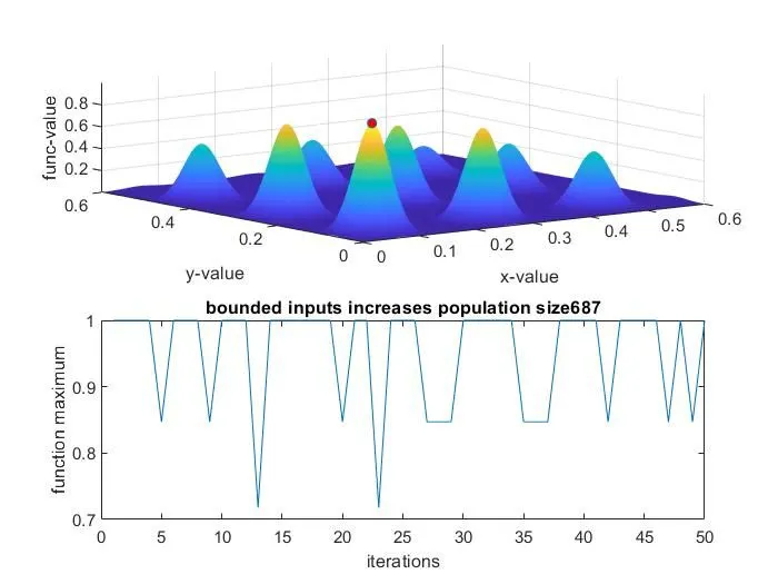
The use of 'population method within bounded input increases the exact value of global maxima.assumed value of population size is 50
conclusion : The global maxima is calculated by populatiob sizing and the plot provide a visual context of the solution and verifies the authenticity of the obtained value