Project 1
Aim : Deals with the development of a forward energy-based fuel consumption model of a conventional vehicle and the main goal of this project is to get familiar with the modeling process, writing scripts in Matlab, modeling in Simulink, analyzing data and generating plots.abulate the fuel economy numbers (kmpl) for UDDS and HWFET cycle. This forms the baseline numbers for comparing with the future hybrid version
Objective:
1) Load the Project1 folder as the Current Folder in Matlab.
2) Run the “Project1_InitFile.m” Matlab script.
3) The provided vehicle Simulink model “Project1_VehicleModel.slx” is incomplete. The engine and vehicle dynamics block contents have been deleted. Build the Simulink blocks by referring to the course lecture and example block images provided. You can run the model and analyze the results using a ‘Scope’ for debugging.
4) Add additional ‘To Workspace’ blocks for transferring the desired Simulink vehicle data into the Matlab workspace.
5) Modify the “Project1_ProcessingFile.m” as per the desired plots and required calculations.
6) Write a project report that contains the following:
Theory: The transport sector has increased about 40% since 1990 but the depletion of petroleum and the increase of pollutants lead the manufacturers to develop other transportation systemsolutions. The Utopian solution would be to replace all the conventional vehicles by Electric Vehicles (EVs) but theirstorage device is limited. An intermediate solution is Hybrid
Electric Vehicles (HEVs) but these vehicles are difficult to analyze and their energy management is complex.
The purpose of this technical paper is to compare two approaches of control strategy (forward and backward)currently used to determine best practices. Since the objectiveis to compare two approaches the studied vehicle will be asimple EV represented This choice allows to be more focused on the comparison and not in the determination of hybrid supervision control, which is difficult to define. So, the work is to compare the Energetic MacroscopicRepresentation (EMR – forward approach) with WarwickPowertrain Simulation Tool for Architectures (WARPSTAR– backward approach).EMR is a graphical description exclusivelybased on physical causality (i.e. integral causality) . This property enables a straightforward deduction of a control scheme that can be implemented in real-time, that is not the case for other graphical descriptions. Such a dynamic modelling highlights energy properties of the power components such as energy storage, energy conversion and energy distribution. Moreover, an inversion-based control canbe systematically deduced from EMR, step-by-step, by
inverting the elements. WARPSTAR is a modelling package for investigation of HEVs architectures. WARPSTAR offers a full range of functionality in one structure, due to thenon-causal approach, facilitating inverse dynamic Calculations. It also has pre-built models of all knownarchitectures, and a component model library to build new .the proposed vehicle model architecture improves modelling flexibility by standardizing and replicating the real physical coupling between model subsystems. This allows for rapid reconfiguration of the model as well as testing and validation of individual component subsystems in isolation. The addition of an external torque source represented the addition of a hybridizing component to the drivetrain. Due to the new VMA, the external torque source was easily incorporated without excessive modification to the existing drivetrain. It has been shown that the proposed modelling methodology is suitable for the simulation of vehicle dynamics closely matching real world driving data. The new VMA can also include complex components such as clutches and torque convertors, accurately accounting for coupling and decoupling within the powertrain system. The use of the Simulink environment rather than a commercial package also benefits the user/developer by giving extra freedom in model development that other commercial packages may not give. Further work is to be completed on full drive cycle analysis using the new flexible architecture. Full validation of the model will also be performed to both conventional and hybrid drivetrain configurations. Development will also be conducted on the hybrid component models such as motor generator units and energy storage systems to improve the accuracy of the input data to the model whilst allowing additional results to be extracted.
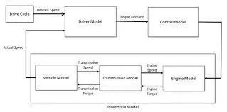
Vehicle Model
Pre - processing
%%%%%%%%%%%%%%%%%%%%%%%%%%%%%%%%%%%%%%%%%%%%%%%%%%%%%%%%%%%%%%%%%%%%%
%% Skill-Lync -> Hybrid Drives Development
% Project 1 - Conventional Vehicle Model
% By - Gunashekar HV
% Description:
%% Initialization File
% Initialization file for loading the variables for the Conventional vehicle simulation model
%% Vehicle Parameters
M = 1500; % Vehicle weight [kg]
Cr = 0.015; % Rolling resistance coefficient
Rw = 0.35; % Rolling radius [m]
Cd = 0.33; % Drag coefficient
Af = 2; % Frontal area [m2]
rhoa = 1.225; % Air density [kg/m3]
Vwind = 0; % Wind velocity [kmph]
g = 9.81; % Gravitational acceleration [m/s2]
theta = 0; % Slope [deg]
myu_road_tire = 1; % Coefficient of friction between tire - road interface
%% Powertrain Parameters
FDR = 3.73; % Final Drive Ratio / Diff Ratio
DiffEff = 0.99; % Differential efficiency (assumed independent of operating conditions)
NumGear = 4; % Number of gears in transmission
TransGear = [1:NumGear]; % Transmission Gears
TransRatio = [3.06, 1.62, 1, 0.7]; % Corresponding Transmission ratios
TransEff = 0.90; % Transmission efficiency (assumed independent of operating conditions)
TC_SR = [0, .5, .6, .7, .8, .87, .92, .94, .96, .97, 1]; % Torque Converter Speed Ratio (Matlab default) -> TurbSpd/PumpSpd
TC_TR = [2.232, 1.5462, 1.4058, 1.2746, 1.1528, 1.0732, 1.0192, 1, 1, 1, 1]; % Torque Converter Torque Ratio (Matlab default) -> TurbTrq/PumpTrq
TC_Cf = 1e-4 * [.72558, .66322, .63463, .59042, .51331, .4144, .29287, .22444, .12186, .04386, 0]; % Torque Converter Capacity Factor (Matlab default) -> PumpTrq/PumpSpd^2 [Nm/rpm^2]
load Vehicle_Data/Engine_data_1_9L_Saturn_95kW
load Vehicle_Data/Trans_Shift_map
%% Driver Parameters
Kp = 10; % P gain for driver PI model
Ki = 1; % I gain for driver PI model
Drive_Cycle_Select = 1; % Drive cycle selection
% Drive cycle values in m/s
if Drive_Cycle_Select == 1
load DriveCycles/UDDS;
elseif Drive_Cycle_Select == 2
load DriveCycles/HWFET;
elseif Drive_Cycle_Select == 3
load DriveCycles/FTP;
elseif Drive_Cycle_Select == 4
load DriveCycles/US06;
elseif Drive_Cycle_Select == 5
load DriveCycles/NEDC;
elseif Drive_Cycle_Select == 6
load DriveCycles/WLTP;
end
time_end = cyc_time(end);
vel_end = cyc_vel(end);
The Drive Cycle can be selected from this MATLAB Script, By changing the variable Drive Cycle_Select to,
1:UDDS
2:HWFET
3:FTP
4:US06
5:NEDC
6:WLTP
Simulink Model :
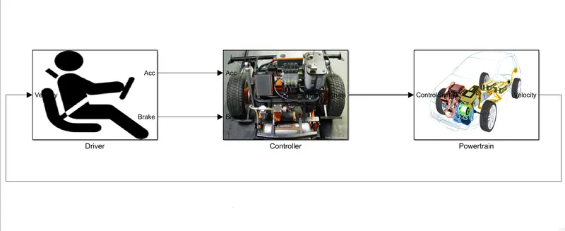
The Simulink model for the convection model is created using 3 main subblocks for the driver model ,control model and powertrain block. The actual vehicle speed is given as feedback to the driver block, and the driver block gives the controller block the required acceleration or brake output, while the controller block provides control signals for engine torque gear shifting and brake torque to the Powertrain model.
Driver Model:
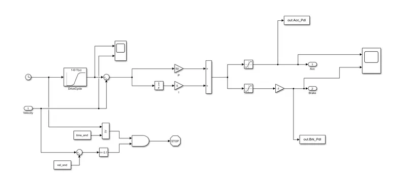
Driver Model is a basic Pl controller that generates accelerator and brake pedal outputs to match the desired and actual vehicle speeds.The Pl controller controls the error between the required drive cycle and actual vehicle speed by providing acceleration and brake pedal output to the controller.
Controller Model:
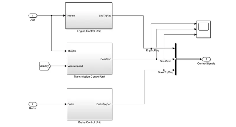
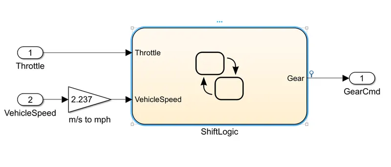
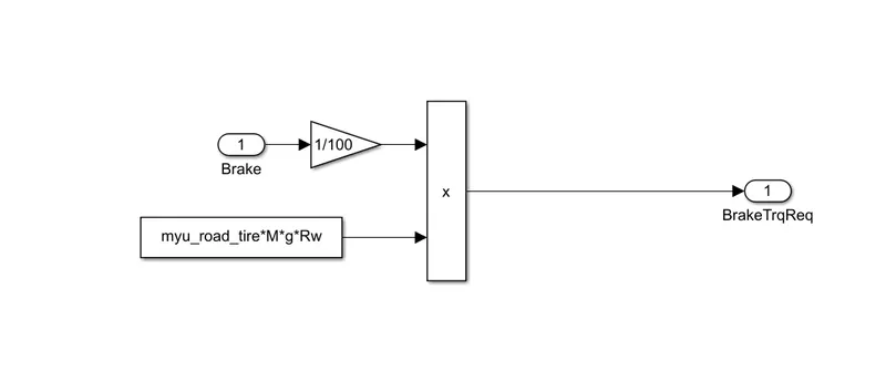
The 'Controller' block is the brains of the vehicle, representing the electronic controls units. Based on the driver inputs, it generates desired engine torque, desired transmission gear and desired brake torque. These inputs are fed to the 'Powertrain' block which represents the drivetrain of the vehicle
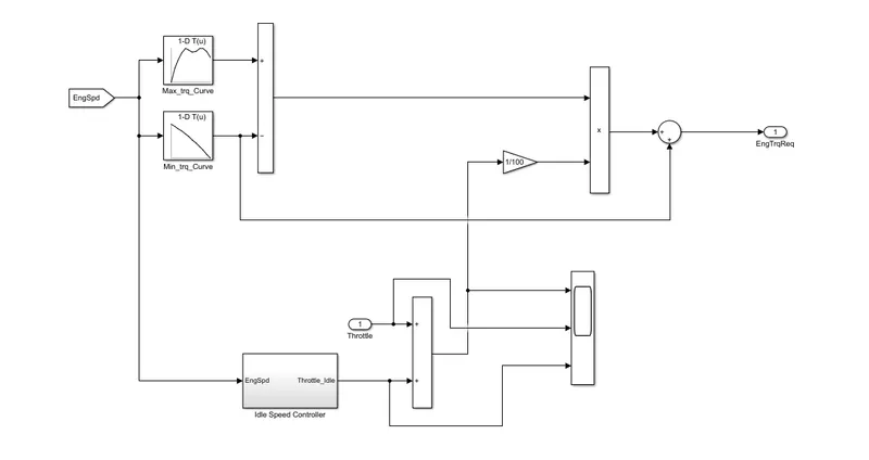
Engine Control Unit:
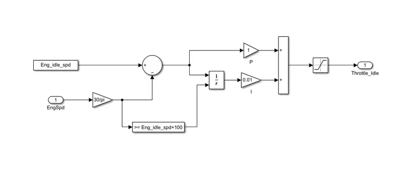
Idle Speed Controller:
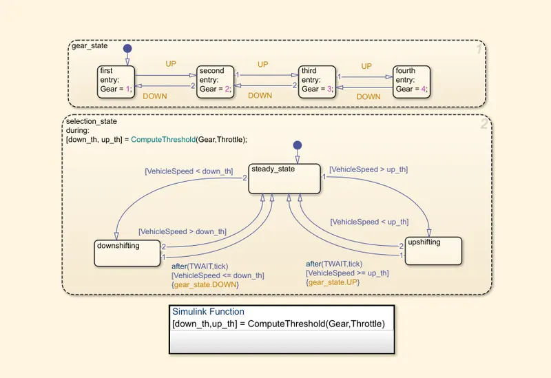
Transmission Control Unit:
Brake Control Unit:
Power Train Model :
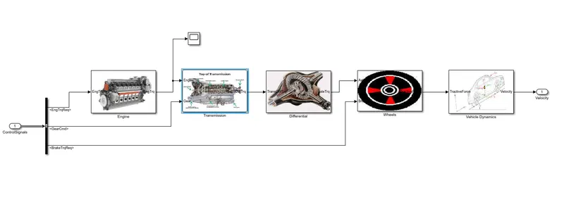
The powertrain is the model, that encompasses every component that converts the power from the engine into mechanical movement. This powertrain model has Engine, Transmission, Differential, Wheels, Vehicle dynamics blocks. From this powertrain block a feedback loop is connected to the driver block to check the different parameters performance and to optimize the vehicle movement. the scope block is connected after the engine block to check the output from the engine, the output from the engine is connected to the transmission block.
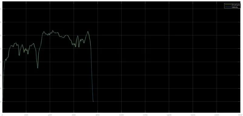
The engine block in the Powertrain model for UDDS fdrive cycle:
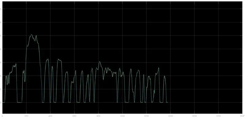
The engine block in the Powertrain model for HWFET fdrive cycle:
Engine Model :
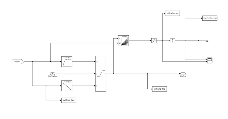
In this engine block, the map-based models are used to model the fuel consumption of the engine. It is based on maximum torque and minimum torque of the controller. In this model have used the look up tables to input the toque data, and the min torque, max torque and the EngTrqReq block is connected to the dynamic saturation input block and the output from the dynamic saturation block is connected to EngTrq block (the output of the engine block) and to 2D look up table (2D look up table get fed the inputs from the dynamic saturation block and the min torque data). The output from the 2d look up table is connected to the saturation block to get the engine fuel rate, and then connected to integrator block to get the fuel consumption.
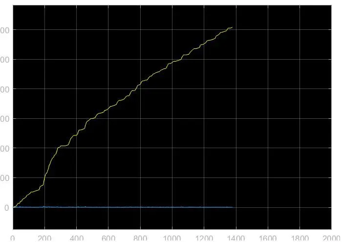
For USSD drive Cycle:
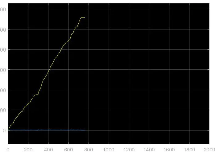
For HWFET drive Cycle:
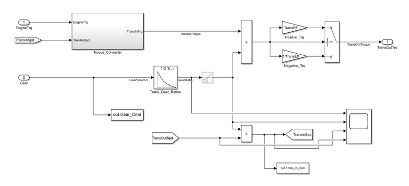
Transmission Model
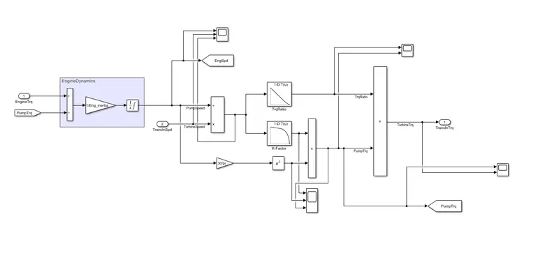
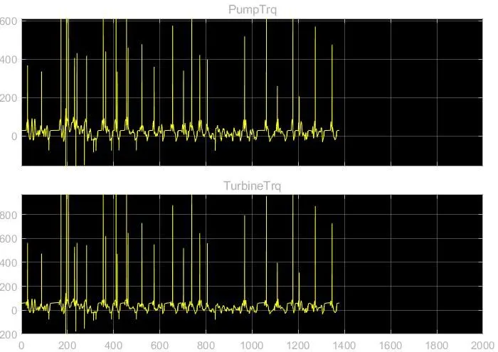
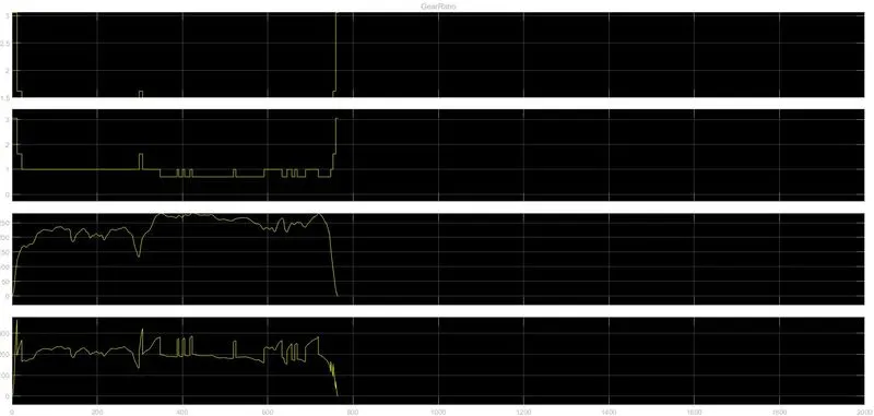
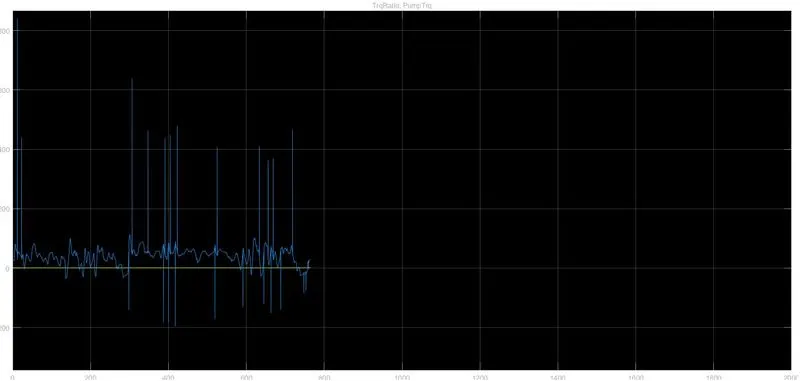
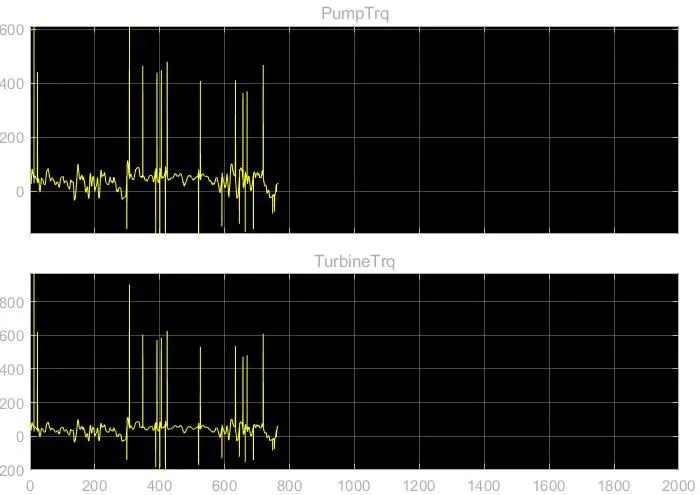
Torque Converter Model
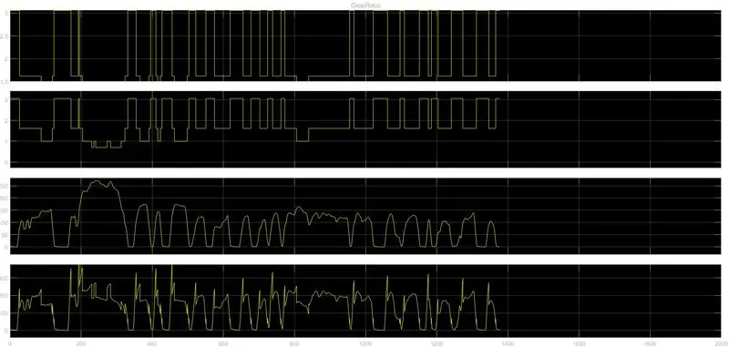
For USSD drive Cycle:
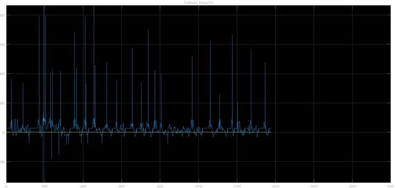
For HWFET drive Cycle:
Differential Model:
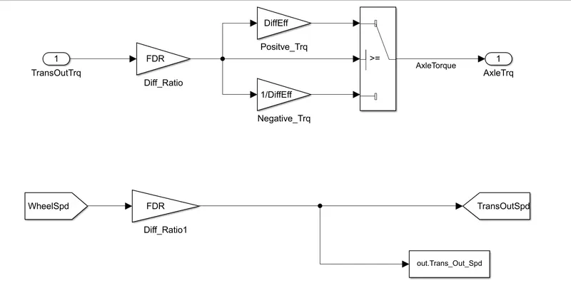
In this differential model, the inputs are fed with the output block of the transmission model (TransOutTrq), this input is multiplied with the differential ratio, the differential ratio get multiplied with output and input torque to get the axle torque. The differential ratio and the transmission torque are greater than the axle torque.
Wheel Model:
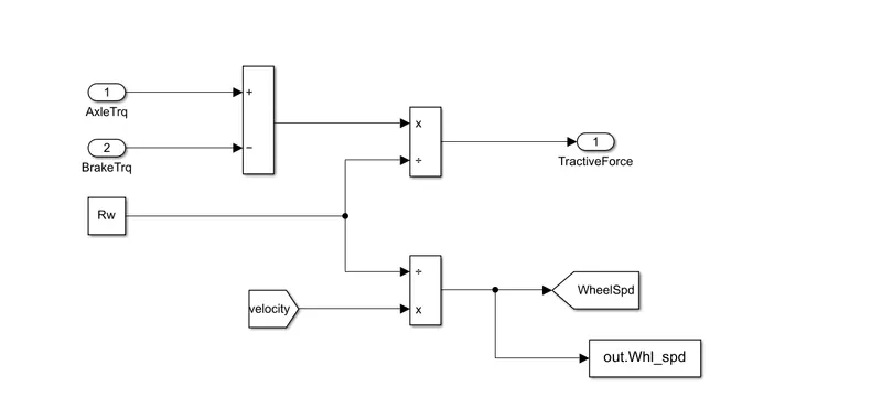
Vehicle Dynamics Model:
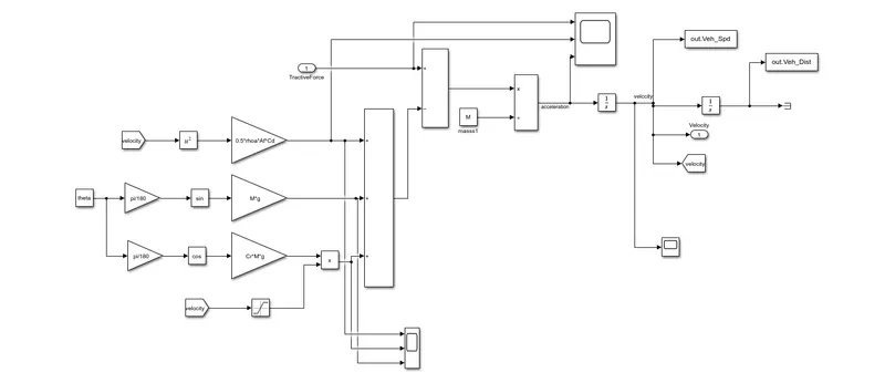
The vehicle dynamics model takes the tractive force as an input. The vehicle dynamics dictates the vehicle speed based on the tractive force and road load. The below equation is used for calculating the road load. The equation is,

where,
pa = Air density [kg/m^3]
Af = Frontal area [m2]
Cd Drag coefficient
Vech = Velocity of vehicle
Vw = Velocity of wind (or) Head wind
Cr= Rolling resistance coefficient
M = Mass [kg]
g= Gravitational force
`theta`= Angel (or) grade
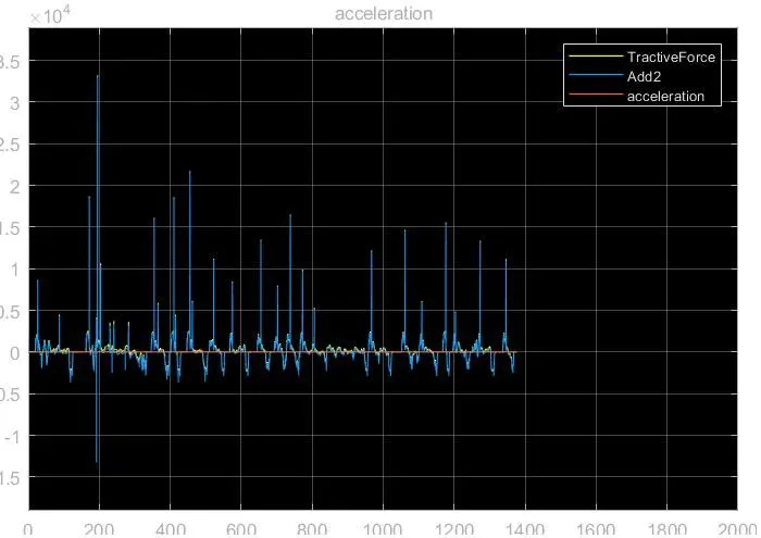
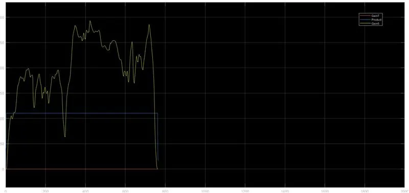
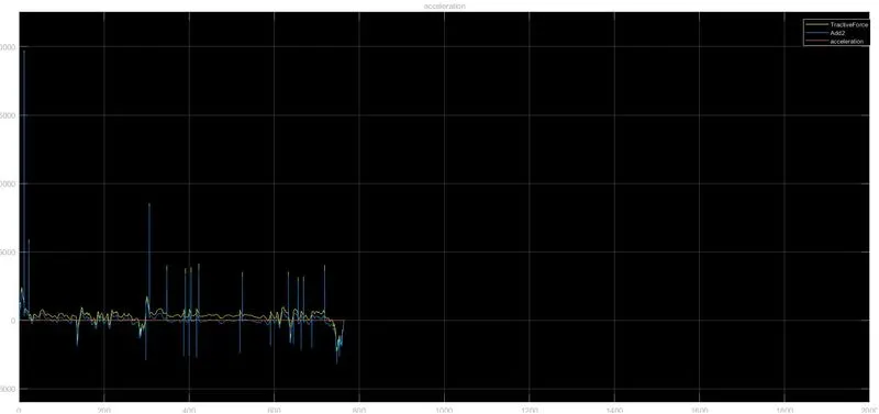
The output from the road load is connected to an add block, another input for add block is tractive force. The mass and sum of tractive force & road load is connected to the divide block to get acceleration, the divide block is connected to integrator block to get vehicle speed. The integrator output (velocity) is connected to one more integrator block to know the vehicle distance. The output velocity is connected to the driver block as an input.
Scope block in vehicle dynamic model For USSD:
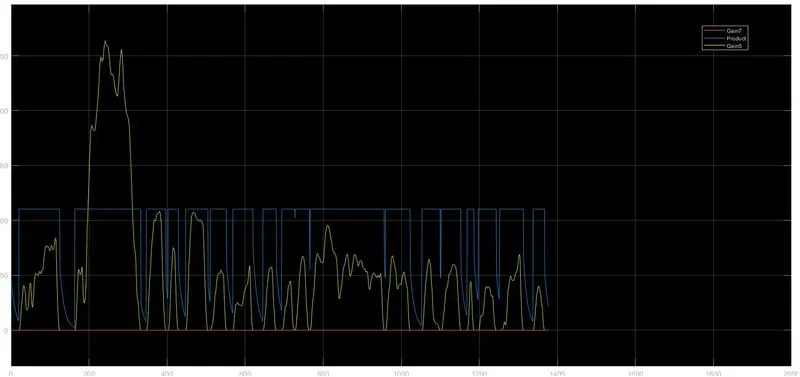
For HWFET drive Cycle:
Once the Simulink vehicle model simulation was done, some data will be sent to the MATLAB workspace with the help of 'To workspace' block. The data from the Simulink model is helps to plot the different parameters of the conventional vehicle in MATLAB.
The below modified program is used to plot the following parameters for both UDDS and HWFET drive cycles
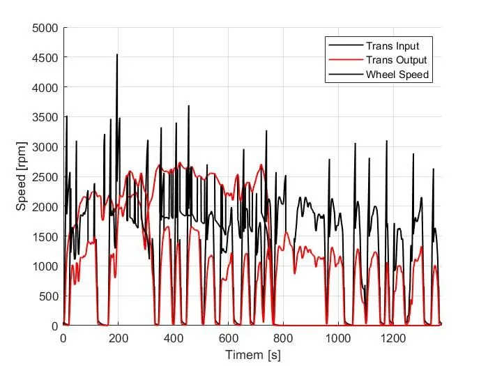
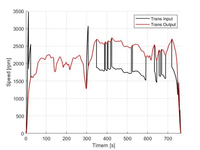
1. Trans input, Trans output and Wheel speed.
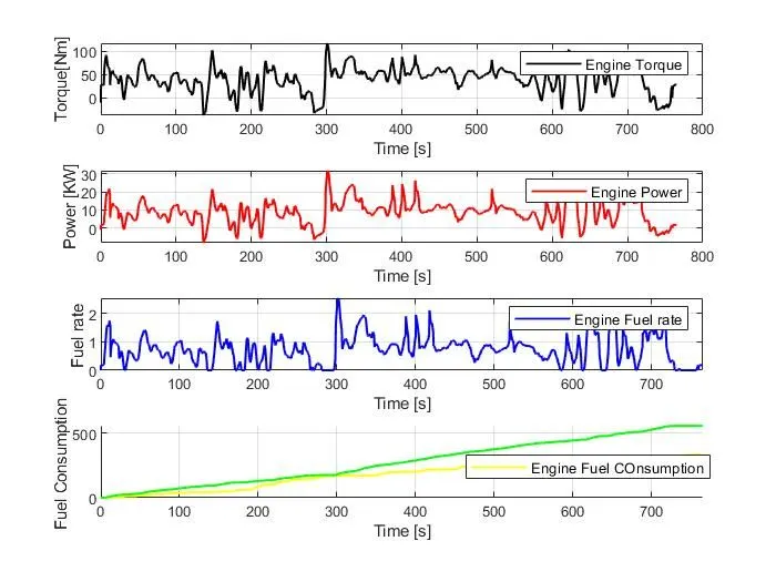
2. Engine Torque, Engine Power, Engine Fuel Rate and Engine Fuel Consumption,
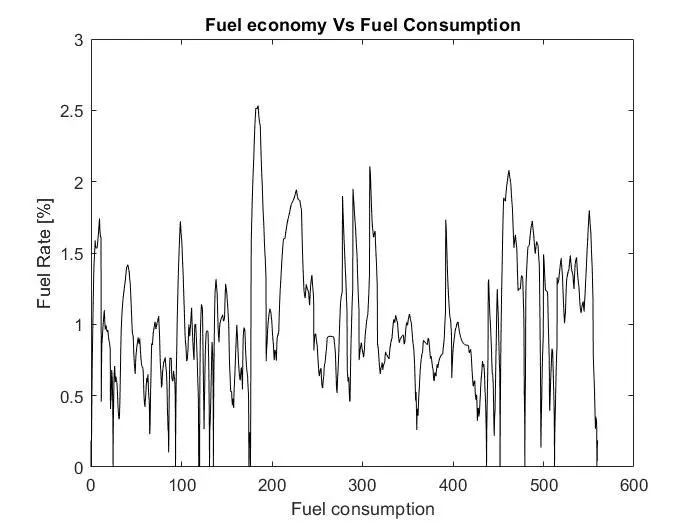
3. Fuel Economy vs Fuel Consumption.
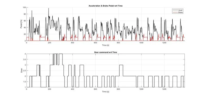
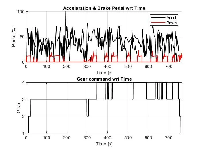
4. Acceleration, Brake pedal and gear command with respect to time.
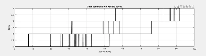
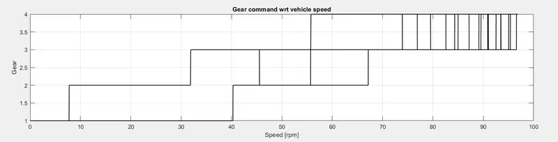
5. Gear command with respect to vehicle speed and distance.
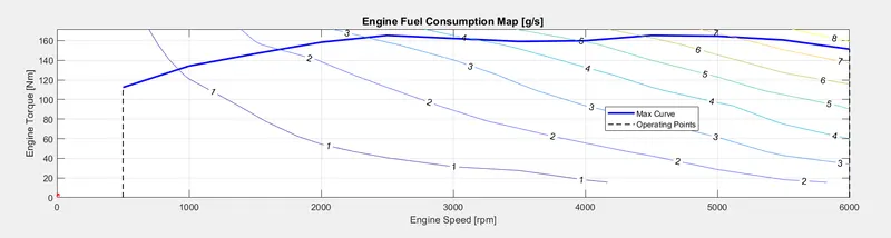
6. Engine Fuel Consumption map [g/s].
Post-Processing File Matlab code:
%%%%%%%%%%%%%%%%%%%%%%%%%%%%%%%%%%%%%%%%%%%%%%%%%%%%%%%%%%%%%%%%%%%%%
%% Skill-Lync -> Hybrid Drives Development
% Project 1 - Conventional Vehicle Model
% By - Gunashekar HV
% Description:
% The following file is to used with the Initialization file and Simulink
% results for post-processing of the data.
% The file is incomplete, has some examples of how the data is imported
% into a readable format, data analysis and plotting examples.
% Based on the project task, use commands in a similar format as given
% below, to analyse the data and generate required plots.
% You can change variable names if desired
%% Post-Processing File
% File for post-processing the Conventional vehicle simulation model data
%% Renaming variables
Time = out.tout;
Acc_Pdl = out.Acc_Pdl; % Accelerator pedal [%]
Brk_Pdl = out.Brk_Pdl; % Brake pedal [%]
Gear_Cmd = out.Gear_Cmd; % Transmission gear
Trans_In_Spd = out.Trans_In_Spd*30/pi; % Transmission input speed [rpm]
Trans_Out_Spd = out.Trans_Out_Spd*30/pi;% Transmission output speed [rpm]
Eng_Trq = out.Eng_Trq; % Engine brake torque [Nm]
Eng_Spd = out.Eng_Spd*30/pi; % Engine speed [rpm]
Eng_Fuel_rate = out.Eng_Fuel_rate; %Engine Fuel rate[gkW]
Eng_Fuel_Consump = out.Eng_Fuel_Consumption; % Engine fuel consumption [g]
Veh_Dist = out.Veh_Dist/1000; % Distance traveled by vehicle [km]
Veh_Spd = out.Veh_Spd*18/5; % Vehicle speed [kmph]
Whl_Spd = out.Whl_spd*30/pi; % Wheel speed [kmph]
Desired_spd = out.Desired_Spd*18/5;
%% Data Analysis
Eng_Pwr= Eng_Spd*pi/30.*Eng_Trq/1000; % Engine brake power [kW]
rho_petrol = 0.7197; % Density of petrol [kg/L]
kmpl = Veh_Dist(end)/(Eng_Fuel_Consump(end)/1000/rho_petrol);% Fuel economy [kmpl]
%% Plotting vehicle characteristics time trace
figure(1)
hold on
grid on
plot(Time, Trans_In_Spd,'linewidth', 1, 'Color', 'black');
plot(Time, Trans_Out_Spd,'linewidth', 1, 'Color', 'red');
xlabel('Timem [s]')
ylabel('Speed [rpm]')
xlim([0, Time(end)]);
legend ('Trans Input','Trans Output','Wheel Speed');
% Plotting Engine speed, Engine Torque, Engine Power, Engine fuel rate, Engine fuel consumption wrt Time
figure(2)
subplot (4,1,1)
plot(Time,Eng_Trq,'linewidth',1,'color','black')
xlabel('Time [s]')
ylabel('Torque[Nm]')
legend ('Engine Torque')
grid on
subplot(4,1,2)
plot(Time,Eng_Pwr, 'linewidth',1,'color', 'red')
xlabel('Time [s]')
ylabel('Power [KW]')
legend('Engine Power')
grid on
subplot(4,1,3)
plot(Time, Eng_Fuel_rate,'linewidth', 1, 'color', 'blue')
xlim([0,Time(end)]);
xlabel('Time [s]')
ylabel('Fuel rate ')
legend('Engine Fuel rate')
grid on
subplot(4,1,4)
hold on
grid on
plot(Time, Eng_Fuel_Consump,'linewidth', 1, 'color', 'yellow')
xlim([0,Time(end)]);
xlabel('Time [s]')
ylabel('Fuel Consumption ')
legend('Engine Fuel COnsumption')
%Plotting fuel economy Vs Engine Fuel consumption
figure(3)
plot(Eng_Fuel_Consump,Eng_Fuel_rate, 'color', 'black')
xlabel('Fuel consumption')
ylabel('Fuel Rate [%]')
title('Fuel economy Vs Fuel Consumption')
% Potting Accelerator pedal, Brake pedal and gear command with respect to time
figure(4)
subplot(2,1,1)
hold on
plot(Time, Acc_Pdl, 'linewidth', 1, 'Color', 'black');
plot(Time, Brk_Pdl, 'linewidth', 1, 'Color', 'red');
xlabel('Time [s]');
ylabel('Pedal [%]')
xlim([0, Time(end)]);
grid on
legend('Accel', 'Brake');
title('Acceleration & Brake Pedal wrt Time')
subplot(2,1,2)
plot(Time, Gear_Cmd, 'linewidth', 1, 'Color', 'black');
xlim([0, Time(end)]);
xlabel('Time [s]');
ylabel('Gear');
grid on
title('Gear command wrt Time')
figure(5)
% Plotting gear command vehicle desired with actual speed
subplot(2,1,1)
plot(Veh_Spd, Gear_Cmd, 'linewidth', 1, 'Color', 'black');
xlabel('Speed [rpm]');
ylabel('Gear');
grid on
title('Gear command wrt vehicle speed')
subplot (2,1,2)
plot(Veh_Dist, Gear_Cmd, 'linewidth', 1, 'Color', 'red');
xlabel('Distance [kmpl]');
ylabel('Gear');
grid on
title('Gear command wrt Distance')
% Plotting engine operating points on engine fuel map figure('Name', 'Engine Operating Points');
hold on
grid on
title('Engine Operating Points', 'fontsize', 12);
p1=plot(Eng_map_spd*30/pi, Eng_max_trq, 'linewidth', 2, 'color', 'r');
p2=line([Eng_map_spd(end)*30/pi Eng_map_spd(end)*30/pi],[0 Eng_max_trq(end)]);
set(p2,'linewidth',1, 'linestyle','--', 'color', 'k');
p3=line([Eng_map_spd(1)*30/pi Eng_map_spd(1)*30/pi],[0 Eng_max_trq(1)]);
set(p3,'linewidth',1, 'linestyle','--', 'color','k');
[c,h] = contour (Eng_map_spd'*30/pi, Eng_map_trq, Eng_fuel_map');
clabel(c,h);
xlabel('Engine Speed [rpm]');
ylabel('Engine Torque [Nm]');
title('Engine Fuel Consumption Map [g/s]');
legend ([p1 p3], {'Max Curve', 'Operating Points'});
axis ([Eng_map_spd (1)*30/pi Eng_map_spd(end)*30/pi 0 Eng_map_trq(end)]);
Plot for USSD and HWFET derive Cycle:
1. Plotting the vehicle characteristic Time Trace, Transmission of IN/OUT and Wheel Speed
For USSD drive Cycle:
For HWFET drive Cycle:
2. Potting the vehicle characteristic Time trace to Engine Torque ,Engine Power,Engine fuel rate and Engine fuel consumption
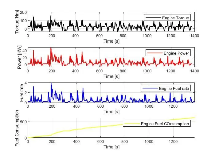
For HWFET drive Cycle:
3.Plotting of Fuel Economy vs Fuel Consumption
For USSD drive Cycle:
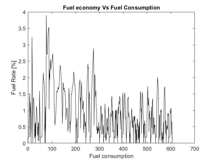
For HWFET drive Cycle:
4.Plotting the Accelaration pedal,break pedal and gear command with respect to time
For USSD drive Cycle:
For HWFET drive Cycle:
5.Plotting Gear command with Vehicle speed and distance:
For USSD drive Cycle:
For HWFET drive Cycle:
PLotting the Engine fuel consumption map:
For USSD drive Cycle:
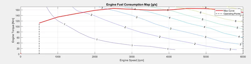
For HWFET drive Cycle: