Project 2

DESCRIPTION:

Description:
As discussed in Lecture 11, Project 2 deals with the development of a forward energy-based fuel consumption model of a P1 hybrid vehicle. This model is based on the conventional vehicle model from Project 1.

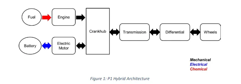
The main goal of this project is to understand the functionality of a P1 hybrid and be able to model it.

Honda Insight motor and battery are considered for this project. Data is taken from ADVISOR data base developed by NREL, USA. Data provided in the project files.

“Project2_InitFile.m” is a Matlab script used to load all the variables required for running the Simulink model and for post-processing. The drive cycle selection is also done here. Before running the Simulink vehicle model, run this initialization script.

Task:

The task of this project is to quantify the improvement in fuel economy numbers for the hybrid vehicle (kmpl), compared to the conventional vehicle, on the urban cycle (UDDS) and highway cycle (HWFET). Also, to analyze and understand the vehicle operating points in terms of engine and motor speed, torque, transmission speeds, pedal positions, gear, distance traveled, battery voltage, current, SoC etc.

To do that, the following steps need to be followed:

1) Load the Project2 folder as the Current Folder in Matlab.
2) Run the “Project2_InitFile.m” Matlab script.
3) Copy the Conventional vehicle Simulink model created for Project 1 in this folder. Figure 1: P1 Hybrid ArchitectureHybrid Drives Development
4) Modify this model into a hybrid vehicle model. The lecture presentations can be used as reference. Battery and Supervisory controller models developed in the assignments can be reused.
5) Add additional ‘To Workspace’ blocks for transferring the desired Simulink vehicle data into the Matlab workspace.
6) Simulate the hybrid model on the desired drive cycles.
7) Write a project report that contains the following:
a. Tabulate the fuel economy numbers (kmpl) for UDDS and HWFET cycle. Compare these numbers with the baseline numbers for conventional vehicle model from Project 1.
b. Plot the time trace for engine, transmission input, transmission output and wheel speed on one plot.
c. Plot engine torque, engine power, fuel rate and fuel consumption using subplots.
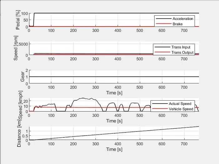
d. Plot accelerator and brake pedal, gear command, vehicle desired and actual speed, vehicle distance using subplots.
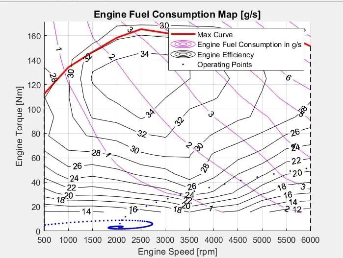
e. Plot the engine operating points on the engine fuel map.
f. Plot motor speed, torque, motor input power using subplots.
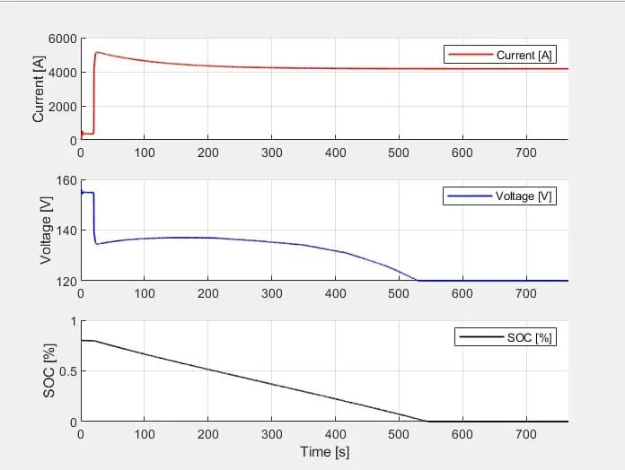
g. Plot pack voltage, current and SoC using subplots.
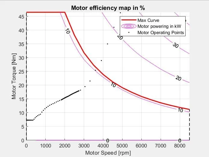
h. Plot the motor operating points on the motor input power map, with the motor max motoring and generating torque curves.
i. Write down appropriate brief comments on each of these plots, describing the vehicle behavior throughout the drive cycle.
j. Generate the plots for both drive cycles

INTRODUCTION:

Crankshaft mounted electric machine or P1 hybird architecture:
The P1 architecture, with the electric machine connected directly to the crankshaft, is the solution adopted by Honda on their first generation Integrated Motor Assist (IMA) technology. The electric motor functions as a generator, during vehicle deceleration, as an engine starter, and as a motor (to assist the engine) during vehicle accelerations.
One of the biggest advantage of this solution is that the electric motor can provide higher torque than the BiSG, since there is no belt limitation (due to slip). However, since there is no speed / torque ratio between the electric machine and crankshaft, the torque requirements on the electric motor can be quite demanding.

Urban Dynamometer Driving Schedule (UDDS):

UDDS stands for Urban Dynamometer Driving Schedule and refers to a United states environmental protection agency mandated dynamometer test on fuel economy that represents city driving conditions which is used for light duty vehicle testing.

It is also known as U.S. FTP-72 (Federal Test Procedure) cycle, LA-4 cycle, in Sweden as A10 or CVS (Constant Volume Sampler) cycle and in Australia as the ADR 27 (Australian Design Rules) cycle.

Though it was originally created as a reference point for fossil fueled vehicles, it is also used to give estimates on how many miles an electric vehicle will travel on a single charge.

Highway Fuel Economy Driving Schedule (HWEFT):

• The "highway" program or Highway Fuel Economy Driving Schedule (HWFET) is defined in 40 CFR 600.I.
• The procedure is updated by adding the "hot start" cycle that repeats the "cold start" cycle of the beginning of the UDDS cycle.
• The average speed is thus different but the maximum speed remains the same as in the UDDS. The weighting factors are 0.43 for the cold start and transient phases together and 0.57 for the hot start phase.
• It uses a warmed-up engine and makes no stops, averaging 48 mph (77 km/h) with a top speed of 60 mph (97 km/h) over a 10- mile (16 km) distance.

Procedure:

• From the given file, download the attachement and change the folder to current folder in matlab.
• Then run the "Project2_InitFile.m” matlab script and enter the correct in and out to select the drive cycle.
• Open simulink and “Project2.slx” and add the changes to blocks by converting the conventional vehicle to P1 hybrid vehicle.

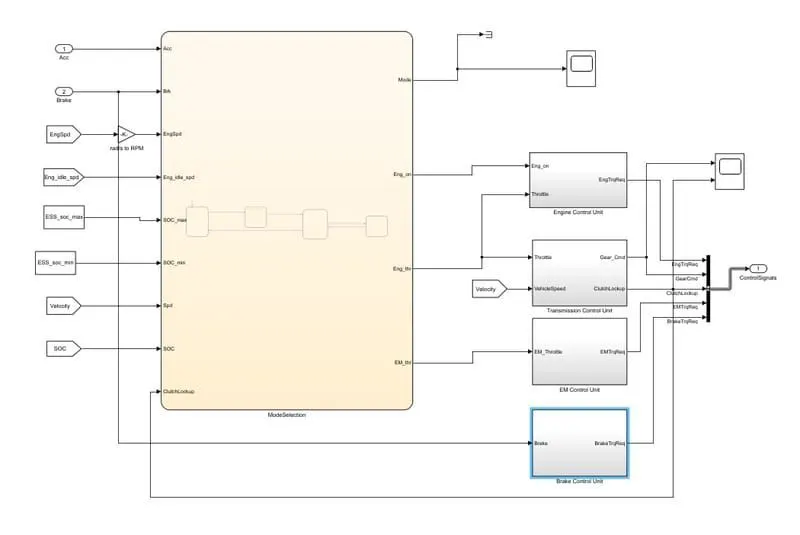
Controller block :

 

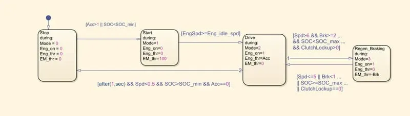
Mode selection chart :

 

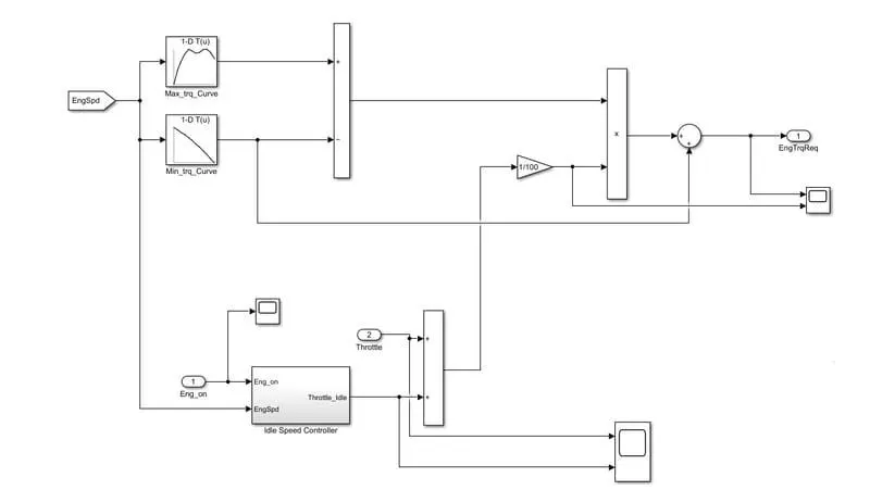
Engine control unit block :

 

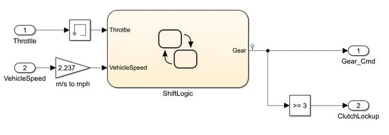
Transmission control unit block :

 

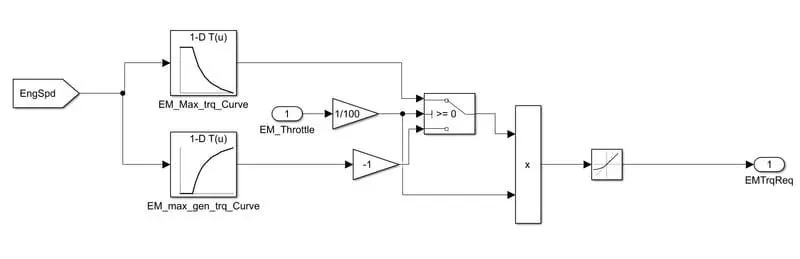
Electric motor control unit block :

 

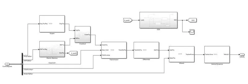
Powertrain block :

 

Electric motor block:

 

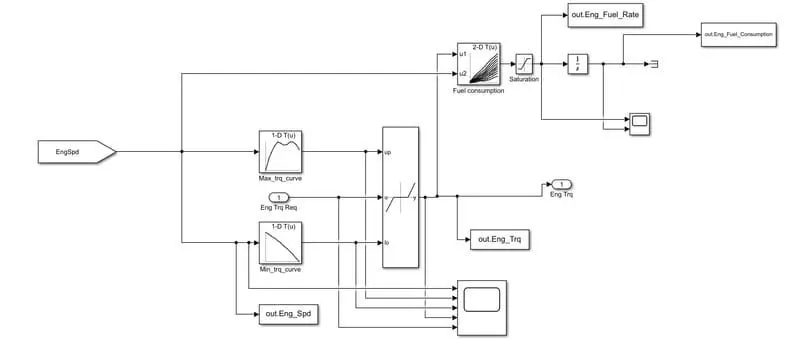
Crankhub block :

 

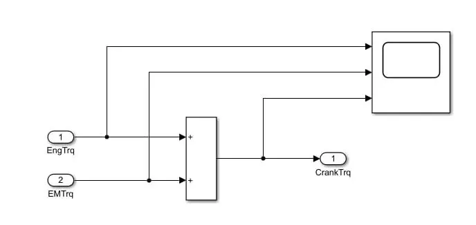
Transmission block :

 

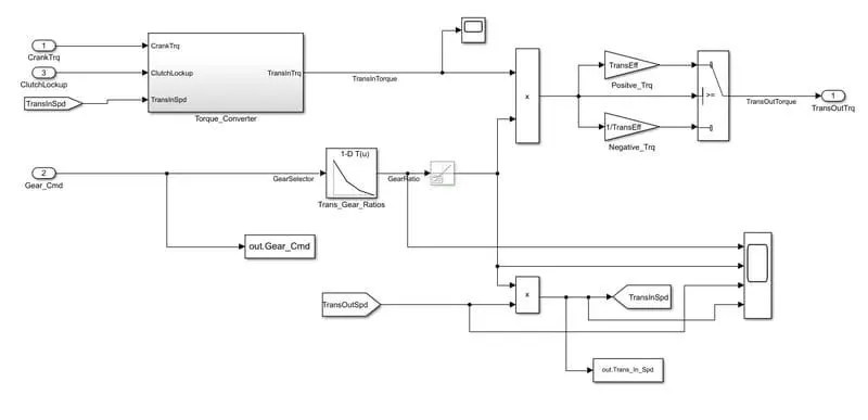
Torque converter block :

 

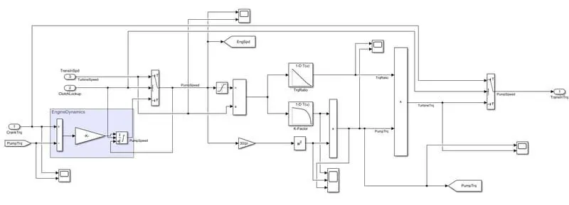
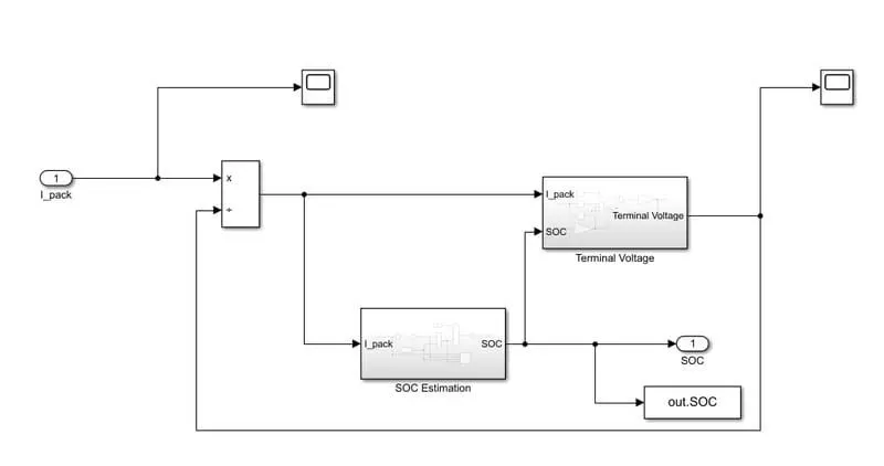
ESS block :

 

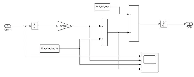
SOC estimation block :

 

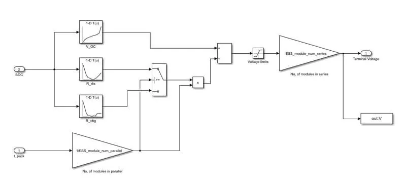
Terminal voltage block :

Program:
Project2_InitFile.m

%% Initialization File
% Initialization file for loading the variables for the Conventional vehicle simulation model

%% Vehicle Parameters
M = 1500; % Vehicle weight [kg]
Cr = 0.015; % Rolling resistance coefficient
Rw = 0.35; % Rolling radius [m]
Cd = 0.33; % Drag coefficient
Af = 2; % Frontal area [m2]
rhoa = 1.225; % Air density [kg/m3]
Vwind = 0; % Wind velocity [kmph]
g = 9.81; % Gravitational acceleration [m/s2]
theta = 0; % Slope [deg]
myu_road_tire = 1; % Coefficient of friction between tire - road interface

%% Powertrain Parameters 
FDR = 3.73; % Final Drive Ratio / Diff Ratio
DiffEff = 0.99; % Differential efficiency (assumed independent of operating conditions)

NumGear = 4; % Number of gears in transmission
TransGear = [1:NumGear]; % Transmission Gears
TransRatio = [3.06, 1.62, 1, 0.7]; % Corresponding Transmission ratios
TransEff = 0.90; % Transmission efficiency (assumed independent of operating conditions)

TC_SR = [0, .5, .6, .7, .8, .87, .92, .94, .96, .97, 1]; % Torque Converter Speed Ratio (Matlab default) -> TurbSpd/PumpSpd 
TC_TR = [2.232, 1.5462, 1.4058, 1.2746, 1.1528, 1.0732, 1.0192, 1, 1, 1, 1]; % Torque Converter Torque Ratio (Matlab default) -> TurbTrq/PumpTrq
TC_Cf = 1e-4 * [.72558, .66322, .63463, .59042, .51331, .4144, .29287, .22444, .12186, .04386, 0]; % Torque Converter Capacity Factor (Matlab default) -> PumpTrq/PumpSpd^2 [Nm/rpm^2]

load Vehicle_Data/Engine_data_1_9L_Saturn_95kW
load Vehicle_Data/Trans_Shift_map
load Vehicle_Data/EM_Honda_Insight_10kW
load Vehicle_Data/ESS_NiMH6
load Vehicle_Data/Pack_Current_test

ESS_init_soc = 0.8;
ESS_soc_max = 0.9;
ESS_soc_min = 0.6;

%% Driver Parameters
Kp = 10; % P gain for driver PI model
Ki = 1; % I gain for driver PI model
Drive_Cycle_Select = 1; % Drive cycle selection

% Drive cycle values in m/s

if Drive_Cycle_Select == 1
load DriveCycles/UDDS;

elseif Drive_Cycle_Select == 2
load DriveCycles/HWFET;

elseif Drive_Cycle_Select == 3
load DriveCycles/FTP;

elseif Drive_Cycle_Select == 4
load DriveCycles/US06;

elseif Drive_Cycle_Select == 5
load DriveCycles/NEDC;

elseif Drive_Cycle_Select == 6
load DriveCycles/WLTP;


end

time_end = cyc_time(end);
vel_end = cyc_vel(end);

set_param('Project_2','DataTypeOverride','Off')

Project2_ProcessingFile:

%% Renaming variables
Time = out.tout;
Acc_Pdl = out.Acc_Pdl; % Accelerator pedal [%]
Brk_Pdl = out.Brk_Pdl; % Brake pedal [%]
Gear_Cmd = out.Gear_Cmd; % Transmission gear
Trans_In_Spd = out.Trans_In_Spd*30/pi; % Transmission input speed [rpm]
Trans_Out_Spd = out.Trans_Out_Spd*30/pi;% Transmission output speed [rpm]
Eng_Trq = out.Eng_Trq; % Engine brake torque [Nm]
Eng_Spd = out.Eng_Spd*30/pi; % Engine speed [rpm]
Eng_Fuel_Consump = out.Eng_Fuel_Consumption; % Engine fuel consumption [g]
Eng_Fuel_Rate= out.Eng_Fuel_Rate;
Veh_Dist = out.Veh_Dist/1000; % Distance traveled by vehicle [km]
Veh_Spd = out.Veh_Spd*18/5; % Vehicle speed [kmph]
Act_Spd=out.Act_Spd; % Actual speed in [kmph]
EMS=out.EM_spd./0.10472;
P=out.ElecPwr;
SOC=out.SOC;
V=out.V;

%% Data Analysis
Eng_Pwr = Eng_Spd.*pi./30.*Eng_Trq./1000; % Engine brake power [kW]
rho_petrol = 0.7197; % Density of petrol [kg/L]
Eff=Eng_eff_map.*100;
Pwr=EM_inpwr_map./1000;
EMT=9.5488.*P./EMS;
kmpl = Veh_Dist(end)/(Eng_Fuel_Consump(end)/1000/rho_petrol); % Fuel economy [kmpl]
Range=P(end)./(Eng_Fuel_Consump(end)*100/1000/rho_petrol);

%% Plotting vehicle characteristics time trace
figure(1)
subplot(5,1,1)
hold on
grid on
plot(Time, Acc_Pdl, 'linewidth', 1, 'Color', 'black');
plot(Time, Brk_Pdl, 'linewidth', 1, 'Color', 'red');
ylabel('Pedal [%]')
xlim([0, Time(end)]);
legend('Acceleration','Brake');
subplot(5,1,2)
hold on
grid on
plot(Time, Trans_In_Spd, 'linewidth', 1, 'Color', 'black');
plot(Time, Trans_Out_Spd, 'linewidth', 1, 'Color', 'red');
ylabel('Speed [rpm]')
xlim([0, Time(end)]);
ylim([0, 6000]);
legend('Trans Input','Trans Output');
subplot(5,1,3)
hold on
grid on
plot(Time, Gear_Cmd, 'linewidth', 1, 'Color', 'black');
xlim([0, Time(end)]);
xlabel('Time [s]');
ylabel('Gear');
subplot(5,1,4)
hold on
grid on
plot(Time, Act_Spd, 'linewidth', 1, 'Color', 'black');
plot(Time, Veh_Spd, 'linewidth', 1, 'Color', 'red');
xlim([0, Time(end)]);
xlabel('Time [s]');
ylabel('Speed [kmph]');
legend('Actual Speed','Vehicle Speed');
subplot(5,1,5)
hold on
grid on
plot(Time,Veh_Dist, 'linewidth', 1, 'Color', 'black');
xlim([0, Time(end)]);
xlabel('Time [s]');
ylabel('Distance [km]');
%% Plotting engine operating points on engine fuel map
figure(2);
hold on
grid on
title('Engine Operating Points','fontsize',12);
p1=plot(Eng_map_spd*30/pi,Eng_max_trq,'linewidth',2,'color','r');
[c,h] = contour(Eng_map_spd'*30/pi,Eng_map_trq,Eng_fuel_map','m');
clabel(c,h);
[c1,h1] = contour(Eng_map_spd'*30/pi,Eng_map_trq,Eff','k');
clabel(c1,h1);
p2=plot(Eng_Spd*30/pi,Eng_Trq,'.','color','b');
p3=line([Eng_map_spd(end)*30/pi Eng_map_spd(end)*30/pi],[0 Eng_max_trq(end)]);
set(p3,'linewidth',1,'linestyle','--','color','k');
xlabel('Engine Speed [rpm]');
ylabel('Engine Torque [Nm]');
title('Engine Fuel Consumption Map [g/s]');
p4 = line([Eng_map_spd(1)*30/pi Eng_map_spd(1)*30/pi],[0 Eng_max_trq(1)]);
set(p4,'linewidth',1,'linestyle','--','color','k');
legend('Max Curve','Engine Fuel Consumption in g/s','Engine Efficiency','Operating Points');
axis([Eng_map_spd(1)*30/pi Eng_map_spd(end)*30/pi 0 Eng_map_trq(end)]);

%% Plotting Motor operating points
figure(3);
hold on
grid on
title('Motor Operating Points','fontsize',12);
p1=plot(EM_map_spd*30/pi,EM_max_trq,'linewidth',2,'color','r');
[c,h] = contour(EM_map_spd'*30/pi,EM_map_trq,Pwr','m');
clabel(c,h);
p2 = plot(EMS*30/pi,EMT,'.','color','b');
set(p2,'linewidth',1,'marker','.','color','k');
p3=line([EM_map_spd(end)*30/pi EM_map_spd(end)*30/pi],[0 EM_max_trq(end)]);
set(p3,'linewidth',1,'linestyle','--','color','k');
p4=line([EM_map_spd(1)*30/pi EM_map_spd(1)*30/pi],[0 EM_max_trq(1)]);
set(p4,'linewidth',1,'linestyle','--','color','k');
xlabel('Motor Speed [rpm]');
ylabel('Motor Torque [Nm]');
title('Motor efficiency map in %');
legend('Max Curve','Motor powering in kW','Motor Operating Points');
axis([EM_map_spd(1)*30/pi EM_map_spd(end)*30/pi 0 EM_map_trq(end)]);

figure(4);
subplot(3,1,1)
hold on
grid on
plot(Time, P, 'linewidth', 1, 'Color', 'r');
xlim([0, Time(end)]);
ylim([0, 6000]);
ylabel('Current [A]')
legend('Current [A]');
subplot(3,1,2)
hold on
grid on
plot(Time, V, 'linewidth', 1, 'Color', 'b');
xlim([0, Time(end)]);
ylabel('Voltage [V]')
legend('Voltage [V]');
subplot(3,1,3)
hold on
grid on
plot(Time, SOC, 'linewidth', 1, 'Color', 'k');
legend('SOC [%]');
xlim([0, Time(end)]);
xlabel('Time [s]');
ylabel('SOC [%]');

%Display calculated fuel economy of vehicle
fprintf('nFuel economy [km/L] : %f kmpl',kmpl);
fprintf('nElectrical drive Range [km] : %f km',Range);

Plots:

Characteristics of Urban Dynamometer Driving Schedule (UDDS):

 

Engine fuel efficiency map:

 

Motor powering map:

 

Battery stats: