Week 3 - Solving second order ODEs
1.Introduction :-
In mathematics a differential equation is an equation thet relatesm one or more functions and there derivatives. in application the functions generally present physical quantities, the derivatives in application the function generally represents physical quantities the derivatives represents there rate change , the differential equations defines a relationship between the two relations are common therefore the differential equations play a prominent role in many desciplines including engineering , physics , economics and biology.
2.Objective :-
To capture the motion of simple pendulum with damper by solving the governing equation for the equation for the motion which basically a second order ODEs an creating an animation using MATLAB.
3.Theory :-
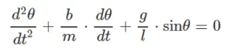
In engineering , ODEs is used to describes the transient behavior of the system. A simple example is pendulum, the way pendulum moves on the Newtons second law is written down, we get second order ODEs that describes the positiob of the 'ball' w,r,t,time. similarly there are hundreds of ODEs that describes the key phenomena and if you havr the ability to solve these equations then you will be able to simulate any of these system.
4.FIXED PARAMETERS :
Length (L) =1 metre,
Mass (m) =1 kg,
Damping coiefficient (b) =0.05.
Acceleration due to gravity (g) =9.81 m/s2.
For Time period = 0-20 sec
Angular displacement=0
Angular velocity=3 rad/sec at time t=0.
5. FUNCTION CODE:
% ODE Function
function dtheta_dt = ode_funs(t,theta,b,g,l,m);
theta1 = theta(1);
theta2 = theta(2);
dtheta1_dt = theta2;
dtheta2_dt = ‐(b/m)*theta2‐(g/l)*sin(theta1);
dtheta_dt = [ dtheta1_dt ; dtheta2_dt];
end
6.EXPLANATION:
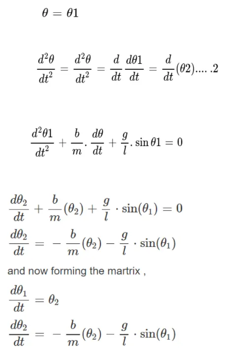
•In this function program, the second-order ODE is simplified to the first-order ODE by introducing the term theta1 & theta2.
•Then theta1 & theta2 is differentiated and the dtheta_dt gives a column matrix.
7.MAIN PROGRAM:
b=0.05;
g=9.81;
l=1;
m=1;
% initial condition
theta_0=[0;3]
% time points
t_span=linspace(0,20,500)';
% solve ODE
[t,results]=ode45(@(t,theta) ode_func(t,theta,b,g,l,m),t_span,theta_0);
figure(1)
plot(t,results(:,1))
hold on
plot(t,results(:,2))
ylabel('velocity')
xlabel('time')
legend('displacement','angular velocity')
hold off
ct=1;
for i=1:length(results(:,1))
x0=0;
y0=0;
x1=l*sin(results(i,1)+pi);
y1=l*cos(results(i,1)+pi);
figure(2)
plot([x0 x1],[y0 y1],'-o','MarkerSize',10,'MarkerFaceColor','r','MarkerEdgeColor','r','linewidth',4)
axis([-2 2 -2 1])
hold on
plot([-1 1],[0 0],[x1 x1],[y1 y1],'linewidth',4,'color','[0 0.3 0]')
M(ct)=getframe(gcf);
ct=ct+1;
hold off
end
% movie & vidiofile
movie(M)
videofile=VideoWriter('pendulum.avi','uncompressed AVI')
open(videofile)
writeVideo(videofile,M)
close(videofile)
8.EXPLANATION:
•In the above program, the fixed parameters are length, mass, damping coefficient, and acceleration due to gravity.
•Time and angle are given as the initial condition.
•In the tspan command, 200 values are taken in between 0 to 20 times period.
•Using the ode 45 command ODE function is introduced.
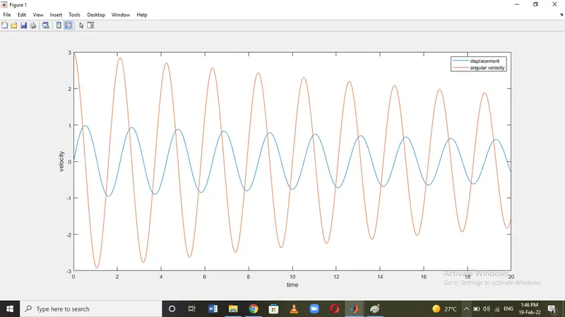
•Using the plot command velocity and displacement is plotted in the y-axis against time in the x-axis.
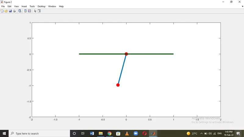
•Using the for loop command the mass at various points and various times are marked in the graph and are plotted.
•Using the movie command the plot is saved as an uncompressed avi file.
9.PLOT:
10.ANIMATION
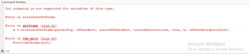
11.ERROR I FACED: