Project 2

Aim:

To get familiar with the modeling process, writing scripts in Matlab, modeling in Simulink, analyzing data and generating plots for development of a forward energy-based fuel consumption model of a P1 hybrid vehicle.The main goal of this project is to understand the functionality of a P1 hybrid and be able to model it.

Objective:

• To evaluate fuel economy numbers (kmpl) and P1 hybrid range for UDDS and HWFET cycle.
• plot time trace for engine, transmission input, transmission output and wheel speed on one plot.
• plot time trace for current,terminal voltage and SOC on one plot.
• Plot engine torque, engine power, fuel rate and fuel consumption.
• Plot accelerator and brake pedal, gear command, vehicle desired and actual speed, vehicle distance using subplots.
• Plot the engine operating points on the engine fuel map.
• Plot motor torque, motor power, motor input power map, with the motor max torque.

Introduction:

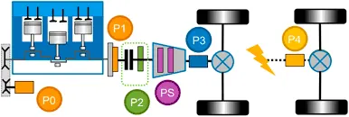
Crankshaft mounted electric machine or P1 hybird architecture:

The P1 architecture, with the electric machine connected directly to the crankshaft, is the solution adopted by Honda on their first generation Integrated Motor Assist (IMA) technology. The electric motor functions as a generator, during vehicle deceleration, as an engine starter, and as a motor (to assist the engine) during vehicle accelerations.

Urban Dynamometer Driving Schedule (UDDS):

• UDDS stands for Urban Dynamometer Driving Schedule and refers to a United states environmental protection agency mandated dynamometer test on fuel economy that represents city driving conditions which is used for light duty vehicle testing.
• It is also known as U.S. FTP-72 (Federal Test Procedure) cycle, LA-4 cycle, in Sweden as A10 or CVS (Constant Volume Sampler) cycle and in Australia as the ADR 27 (Australian Design Rules) cycle.
• Though it was originally created as a reference point for fossil fueled vehicles, it is also used to give estimates on how many miles an electric vehicle will travel on a single charge.

Highway Fuel Economy Driving Schedule (HWEFT):

• The "highway" program or Highway Fuel Economy Driving Schedule (HWFET) is defined in 40 CFR 600.I.
• The procedure is updated by adding the "hot start" cycle that repeats the "cold start" cycle of the beginning of the UDDS cycle. The average speed is thus different but the maximum speed remains the same as in the UDDS. The weighting factors are 0.43 for the cold start and transient phases together and 0.57 for the hot start phase.
• It uses a warmed-up engine and makes no stops, averaging 48 mph (77 km/h) with a top speed of 60 mph (97 km/h) over a 10-mile (16 km) distance.

Procedure:

• From the given file, download the attachement and change the folder to current folder in matlab.
• Then run the "Project2_InitFile.m” matlab script and enter the correct in and out to select the drive cycle.
• Open simulink and “Project2.slx” and add the changes to blocks by converting the conventional vehicle to P1 hybrid vehicle.

Controller block :

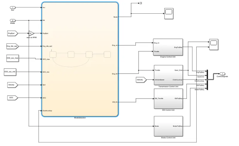
• Add mode selection chart by using the state flow chart in week 10 challenge with proper inputs and outputs as mentioned below.
• Add input block, From workspace block, From block and unit conversion using gain block.
• Connect the output to desired control units and control bus to powertrain block.

Mode selection chart :

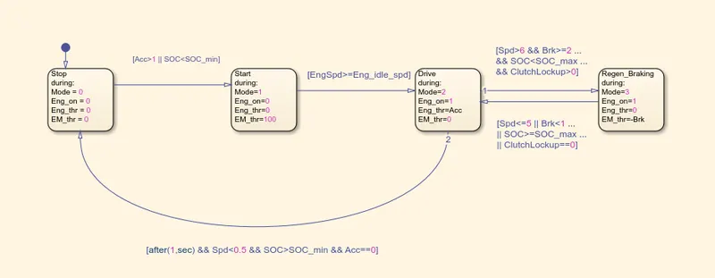
• Mode selection has been driven from start, drive, regen braking and stop.
• Inputs as acceleration, SOC, Engine speed and braking from driver unit.
• Output should be connected to controller units like Engine, electric motor, transmission and brake unit.

Engine control unit block :

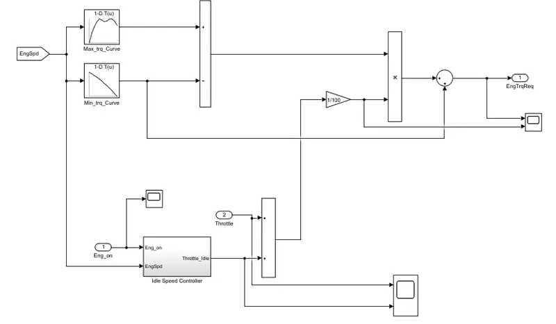
• Engine control unit has been altered by engine on function to idle speed controller unit.
• While engine on was input the idle speed controller creates necessary speed to idle the engine.

Idle speed controller block :

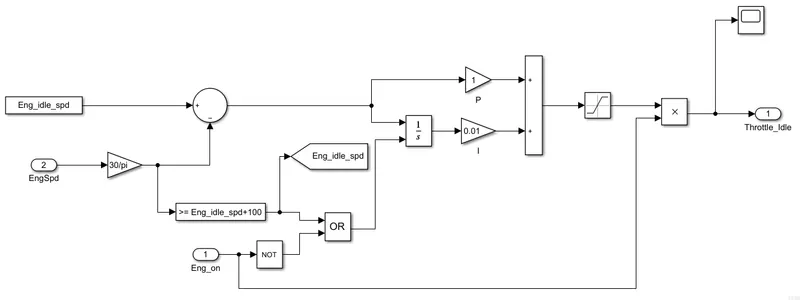
• Using Not gate block the engine on input block generates input to engine to generate idle speed to engine.

Transmission control unit block :

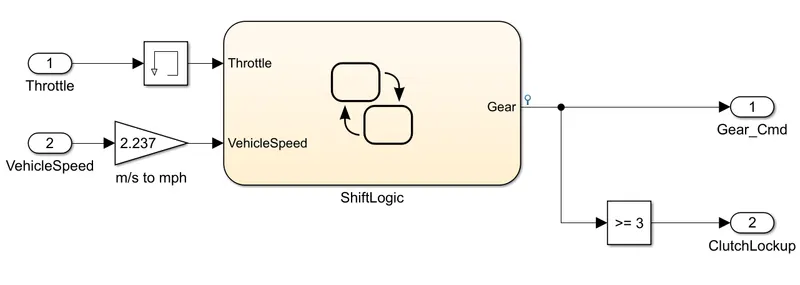
• Use memory block to apply an one integration step delay. The output is the previous input value.
• Use clutch lock up output by using greater than or equal to gear 3.

Electric motor control unit block :

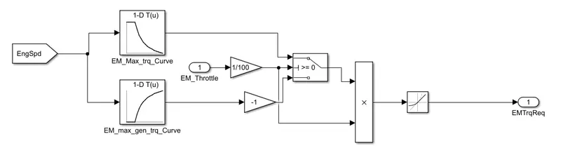
• Electric motor control unit has been generated using engine controller unit.
• Look up table for motor maximum torque curve and maximum generator torque curve with inputs motor speed map, motor torque map and motor input power map.
• Input for unit is motor throttle and output motor torque requirement.

Powertrain block :

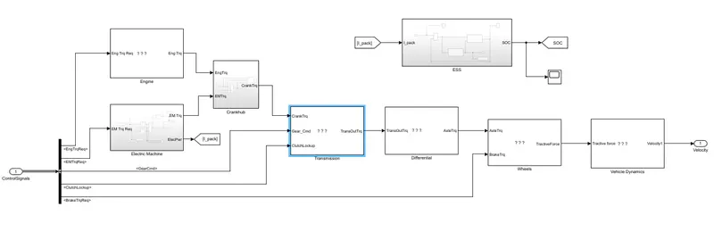
• The powertrain block is updated by electric motor block, crankhub block and battery block.

Electric motor block

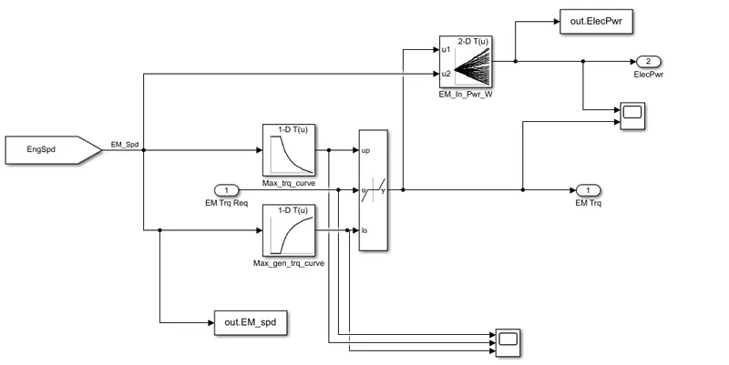
• Use engine block to create except replica as electric motor block.
• Alter the input values as motor speed, motor torque, motor input power map and motor generator torque.
• output as motor torque and eletric power.

Crankhub block :

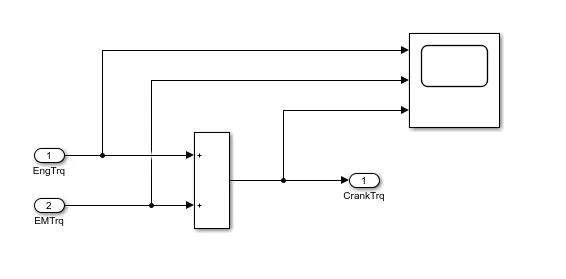
• Crank hub is used to merge both the engine and motor torque with output driven to crank torque.

Transmission block :

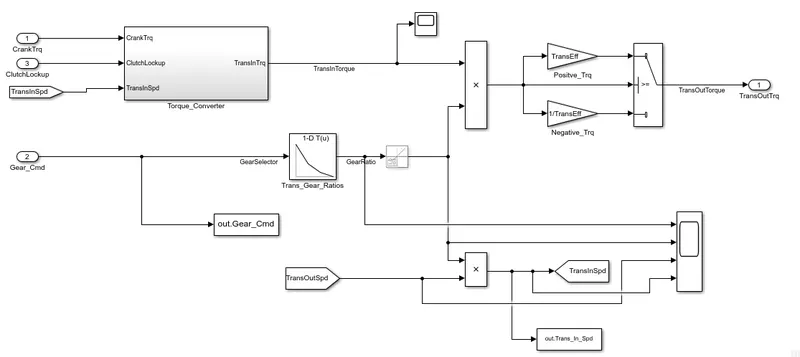
• Transmission block is altered by clutch look up command to transmission unit.

Torque converter block :

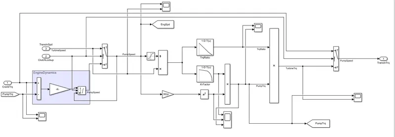
• The lock up clutch is installed on the turbine hub, in front of the turbine. The dampening spring absorbs the torsional force upon clutch engagement to prevent shock transfer. The friction material bonded to the lock up piston is the same as that used on the multiplate clutch discs in the transmission.

ESS block :

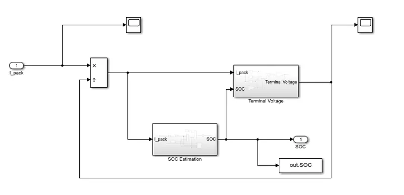
• Battery unit is placed in the powertrain unit.
• Use the simulink block from week 9 challenge.

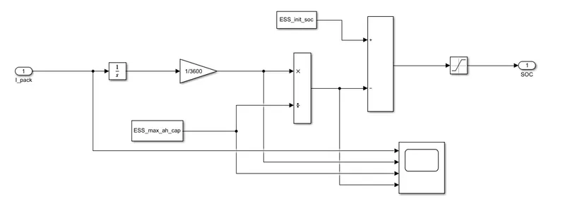
SOC estimation block :

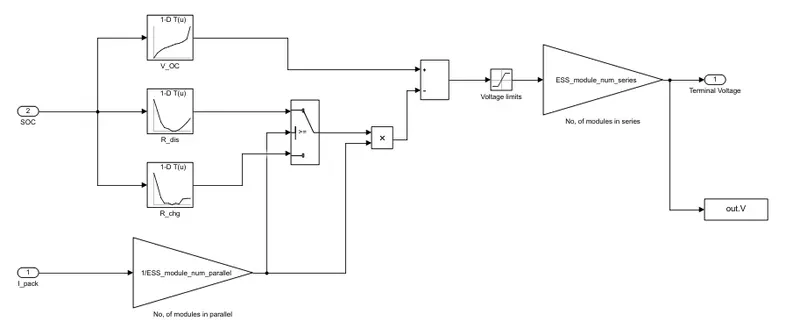
Terminal voltage block :

• Open and modify the “Project2_ProcessingFile.m” as for entered plots and workspace blocks.
• Run the program in following sequence "Project2_InitFile.m”, “Project2.slx” and “Project2_ProcessingFile.m”.
• Verify the genearted output plots.

Program:

Project2_InitFile.m

%% Initialization File
% Initialization file for loading the variables for the Conventional vehicle simulation model

%% Vehicle Parameters
M = 1500;       % Vehicle weight [kg]
Cr = 0.015;     % Rolling resistance coefficient
Rw = 0.35;      % Rolling radius [m]
Cd = 0.33;      % Drag coefficient
Af = 2;         % Frontal area [m2]
rhoa = 1.225;   % Air density [kg/m3]
Vwind = 0;      % Wind velocity [kmph]
g = 9.81;       % Gravitational acceleration [m/s2]
theta = 0;      % Slope [deg]
myu_road_tire = 1; % Coefficient of friction between tire - road interface

%% Powertrain Parameters 
FDR = 3.73;                         % Final Drive Ratio / Diff Ratio
DiffEff = 0.99;                     % Differential efficiency (assumed independent of operating conditions)

NumGear = 4;                        % Number of gears in transmission
TransGear = [1:NumGear];            % Transmission Gears
TransRatio = [3.06, 1.62, 1, 0.7];  % Corresponding Transmission ratios
TransEff = 0.90;                    % Transmission efficiency (assumed independent of operating conditions)

TC_SR = [0, .5, .6, .7, .8, .87, .92, .94, .96, .97, 1];   % Torque Converter Speed Ratio (Matlab default) -> TurbSpd/PumpSpd  
TC_TR = [2.232, 1.5462, 1.4058, 1.2746, 1.1528, 1.0732, 1.0192, 1, 1, 1, 1];   % Torque Converter Torque Ratio (Matlab default) -> TurbTrq/PumpTrq
TC_Cf = 1e-4 * [.72558, .66322, .63463, .59042, .51331, .4144, .29287, .22444, .12186, .04386, 0]; % Torque Converter Capacity Factor (Matlab default) -> PumpTrq/PumpSpd^2 [Nm/rpm^2]

load Vehicle_Data/Engine_data_1_9L_Saturn_95kW
load Vehicle_Data/Trans_Shift_map
load Vehicle_Data/EM_Honda_Insight_10kW
load Vehicle_Data/ESS_NiMH6

ESS_init_soc = 0.8;
ESS_soc_max = 0.9;
ESS_soc_min = 0.6;

%% Driver Parameters
Kp = 10;                    % P gain for driver PI model
Ki = 1;                     % I gain for driver PI model
Drive_Cycle_Select = 2;     % Drive cycle selection

% Drive cycle values in m/s

if Drive_Cycle_Select == 1
    load DriveCycles/UDDS;
    
elseif Drive_Cycle_Select == 2
    load DriveCycles/HWFET;
    
elseif Drive_Cycle_Select == 3
    load DriveCycles/FTP;
    
elseif Drive_Cycle_Select == 4
    load DriveCycles/US06;
    
elseif Drive_Cycle_Select == 5
    load DriveCycles/NEDC;
    
elseif Drive_Cycle_Select == 6
    load DriveCycles/WLTP;
    
 
end

time_end = cyc_time(end);
vel_end = cyc_vel(end);

set_param('Project_2','DataTypeOverride','Off')

Project2.slx

https://drive.google.com/file/d/15P2MOoix3E2gHJUCqB-kTjy10QgtmYTg/view?usp=sharing

Project2_ProcessingFile.m

%% Renaming variables
Time = out.tout;
Acc_Pdl = out.Acc_Pdl;          % Accelerator pedal [%]
Brk_Pdl = out.Brk_Pdl;          % Brake pedal [%]
Gear_Cmd = out.Gear_Cmd;        % Transmission gear
Trans_In_Spd = out.Trans_In_Spd*30/pi;  % Transmission input speed [rpm]
Trans_Out_Spd = out.Trans_Out_Spd*30/pi;% Transmission output speed [rpm]
Eng_Trq = out.Eng_Trq;          % Engine brake torque [Nm]
Eng_Spd = out.Eng_Spd*30/pi;    % Engine speed [rpm]
Eng_Fuel_Consump = out.Eng_Fuel_Consumption;    % Engine fuel consumption [g]
Eng_Fuel_Rate= out.Eng_Fuel_Rate;
Veh_Dist = out.Veh_Dist/1000;   % Distance traveled by vehicle [km]
Veh_Spd = out.Veh_Spd*18/5;     % Vehicle speed [kmph]
Act_Spd=out.Act_Spd;          % Actual speed in [kmph]
EMS=out.EM_spd./0.10472;
P=out.ElecPwr;
SOC=out.SOC;
V=out.V;

%% Data Analysis
Eng_Pwr = Eng_Spd.*pi./30.*Eng_Trq./1000;   % Engine brake power [kW]
rho_petrol = 0.7197;                    % Density of petrol [kg/L]
Eff=Eng_eff_map.*100;
Pwr=EM_inpwr_map./1000;
EMT=9.5488.*P./EMS;
kmpl = Veh_Dist(end)/(Eng_Fuel_Consump(end)/1000/rho_petrol);    % Fuel economy [kmpl]
Range=P(end)./(Eng_Fuel_Consump(end)*100/1000/rho_petrol);

%% Plotting vehicle characteristics time trace
figure(1)
subplot(5,1,1)
hold on
grid on
plot(Time, Acc_Pdl, 'linewidth', 1, 'Color', 'black');
plot(Time, Brk_Pdl, 'linewidth', 1, 'Color', 'red');
ylabel('Pedal [%]')
xlim([0, Time(end)]);
legend('Acceleration','Brake');
subplot(5,1,2)
hold on
grid on
plot(Time, Trans_In_Spd, 'linewidth', 1, 'Color', 'black');
plot(Time, Trans_Out_Spd, 'linewidth', 1, 'Color', 'red');
ylabel('Speed [rpm]')
xlim([0, Time(end)]);
ylim([0, 6000]);
legend('Trans Input','Trans Output');
subplot(5,1,3)
hold on
grid on
plot(Time, Gear_Cmd, 'linewidth', 1, 'Color', 'black');
xlim([0, Time(end)]);
xlabel('Time [s]');
ylabel('Gear');
subplot(5,1,4)
hold on
grid on
plot(Time, Act_Spd, 'linewidth', 1, 'Color', 'black');
plot(Time, Veh_Spd, 'linewidth', 1, 'Color', 'red');
xlim([0, Time(end)]);
xlabel('Time [s]');
ylabel('Speed [kmph]');
legend('Actual Speed','Vehicle Speed');
subplot(5,1,5)
hold on
grid on
plot(Time,Veh_Dist, 'linewidth', 1, 'Color', 'black');
xlim([0, Time(end)]);
xlabel('Time [s]');
ylabel('Distance [km]');

%% Plotting engine operating points on engine fuel map
figure(2);
hold on
grid on
title('Engine Operating Points','fontsize',12);
p1=plot(Eng_map_spd*30/pi,Eng_max_trq,'linewidth',2,'color','r');
[c,h] = contour(Eng_map_spd'*30/pi,Eng_map_trq,Eng_fuel_map','m');
clabel(c,h);
[c1,h1] = contour(Eng_map_spd'*30/pi,Eng_map_trq,Eff','k');
clabel(c1,h1);
p2=plot(Eng_Spd*30/pi,Eng_Trq,'.','color','b');
p3=line([Eng_map_spd(end)*30/pi Eng_map_spd(end)*30/pi],[0 Eng_max_trq(end)]);
set(p3,'linewidth',1,'linestyle','--','color','k');
xlabel('Engine Speed [rpm]');
ylabel('Engine Torque [Nm]');
title('Engine Fuel Consumption Map [g/s]');
p4 = line([Eng_map_spd(1)*30/pi Eng_map_spd(1)*30/pi],[0 Eng_max_trq(1)]);
set(p4,'linewidth',1,'linestyle','--','color','k');
legend('Max Curve','Engine Fuel Consumption in g/s','Engine Efficiency','Operating Points');
axis([Eng_map_spd(1)*30/pi Eng_map_spd(end)*30/pi 0 Eng_map_trq(end)]);

%% Plotting Motor operating points
figure(3);
hold on
grid on
title('Motor Operating Points','fontsize',12);
p1=plot(EM_map_spd*30/pi,EM_max_trq,'linewidth',2,'color','r');
[c,h] = contour(EM_map_spd'*30/pi,EM_map_trq,Pwr','m');
clabel(c,h);
p2 = plot(EMS*30/pi,EMT,'.','color','b');
set(p2,'linewidth',1,'marker','.','color','k');
p3=line([EM_map_spd(end)*30/pi EM_map_spd(end)*30/pi],[0 EM_max_trq(end)]);
set(p3,'linewidth',1,'linestyle','--','color','k');
p4=line([EM_map_spd(1)*30/pi EM_map_spd(1)*30/pi],[0 EM_max_trq(1)]);
set(p4,'linewidth',1,'linestyle','--','color','k');
xlabel('Motor Speed [rpm]');
ylabel('Motor Torque [Nm]');
title('Motor efficiency map in %');
legend('Max Curve','Motor powering in kW','Motor Operating Points');
axis([EM_map_spd(1)*30/pi EM_map_spd(end)*30/pi 0 EM_map_trq(end)]);

figure(4);
subplot(3,1,1)
hold on
grid on
plot(Time, P, 'linewidth', 1, 'Color', 'r');
xlim([0, Time(end)]);
ylim([0, 6000]);
ylabel('Current [A]')
legend('Current [A]');
subplot(3,1,2)
hold on
grid on
plot(Time, V, 'linewidth', 1, 'Color', 'b');
xlim([0, Time(end)]);
ylabel('Voltage [V]')
legend('Voltage [V]');
subplot(3,1,3)
hold on
grid on
plot(Time, SOC, 'linewidth', 1, 'Color', 'k');
legend('SOC [%]');
xlim([0, Time(end)]);
xlabel('Time [s]');
ylabel('SOC [%]');

%Display calculated fuel economy of vehicle
fprintf('\nFuel economy [km/L] : %f kmpl',kmpl);
fprintf('\nElectrical drive Range [km] : %f km',Range);

Plots:

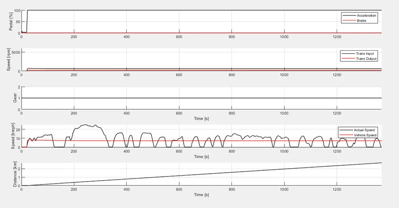
Characteristics of Urban Dynamometer Driving Schedule (UDDS):

• UDDS cycle has desired velocity in uneven manner and the change in controls, outputs differ varyingly.
• Accelerator and brake Pedal percentage with respect to time trace is plotted below in subplot 1. Accelerator pedal is non-linear increasing at some points and also the brake pedal is applied at uneven points but the percentage of pedals be similar after a point which is not so high as the pedal percentage appears linear in map.
• The transmission input and output speed is flat in graph but trans-input speed is greater than trans-ouput speed due to engine operating speed as referred in subplot 2. From this we can see that there requires a clutch to engage, disengage the tranmission for that speed. The time trace to attain that speed in both input and output is high.
• Gear command is linear as referred in subplot 3.
• Comparing the desired velocity of the UDDS cycle over actual vehicle velocity in subplot 4, it has huge difference as the curve for desired velocity is varying at different speeds. The actual velocity of vehicle is smoothly increasing and decreasing which is not evident as desired velocity.
• Referring to subplot 5, the distance travelled by any vehicle always increases linearly in even manner.

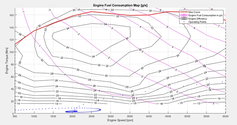
Engine fuel efficiency map:

• Engine fuel efficiency map is genearted using engine speed in rpm and engine torque in Nm.
• The comtours function is used to create the engine fuel consumption in g/s.
• The map also has maximum torque curve and engine operating points in it.
• The speed of the vehicle ranges from 500 rpm to 6000 rpm.
• The torque generated is ranges from 0 Nm to 170 Nm(approx.)
• The maximum torque curve generates at a speed of 500 rpm and 110 Nm. As well as terminates at speed of 6000 rpm and 150 Nm.
• The maximum torque generated at 165.4 Nm.
• Engine fuel consumption ranges from 1 to 8 g/s. At high speed and high torque, the fuel consumption is also high as 8 g/s.
• The plot has engine efficiency i.e. mileage from 12 to 34%.
• Engine operating condition starts at high speed and zero torque. If we look closely the engine operating condition goes beyond its speed range and the graph line reverses. Engine operating condition is non-linear upto a point, torque increases non-linearly and decreases after the speed range.

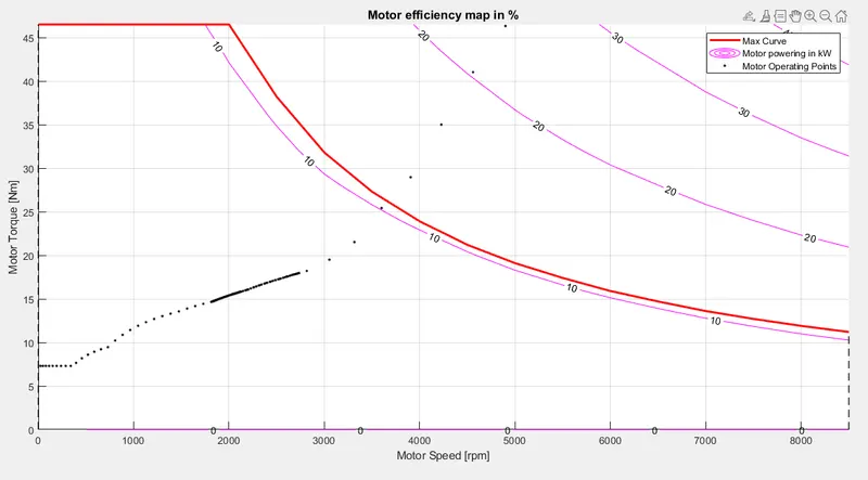
Motor powering map:

• Motor powering map is genearted using motor speed in rpm and motor torque in Nm.
• The contour function is used to create the motor powering map.
• The map also has maximum torque curve and motor operating points in it.
• The speed of the motor ranges from 500 rpm to 8500 rpm.
• The torque generated is ranges from 0 Nm to 67.5 Nm(approx.)
• The maximum torque curve generates at a speed of 500 rpm and 67.5 Nm. As well as terminates at speed of 8500 rpm and 11.2 Nm.
• The maximum torque generated at 67.5 Nm.
• Motor powering ranges from 10 to 40 kW. At high speed and low torque, the power consumption is also high as 40 kW.
• Negative power is plotted which indicates regenerative power from braking of 10 to 20 kW.
• Motor operating condition starts at low speed and low torque. If we look closely the motor operating condition frequently operates at speed range and the graph line steeply increases upto torque of 67.5 Nm and speed of 6970 rpm. The motor delivers high torque and high speed at which the transmission delivers a minmum of it due to torque conversion in crank hub.

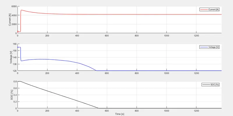
Battery stats:

• Battery delivers power to the hybrid system with terminal voltage and current,
• Battery capacity is measured by state of charge in percentage.
• Time trace of current is 5.120 mA at 24.2 sec and steadily maintains at 4 mA to rest of the cycle.
• Time trace of voltage is 156 V at 0.36 sec and decreases steeply to 134.6 V.
• After which the voltage slowly reaches to 120 V and maintains it till the end of cycle.
• Time trace of SOC is 80% at start maintains till 14 sec and decreases to 0 at 545 sec.

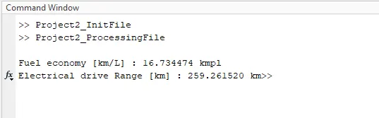
Fuel economy:

From the workspace, we can see the fuel economy of vehicle for UDDS cyce is 16.734474 kmpl and the range of EV is 259.261520 km.

Highway Fuel Economy Driving Schedule (HWEFT):

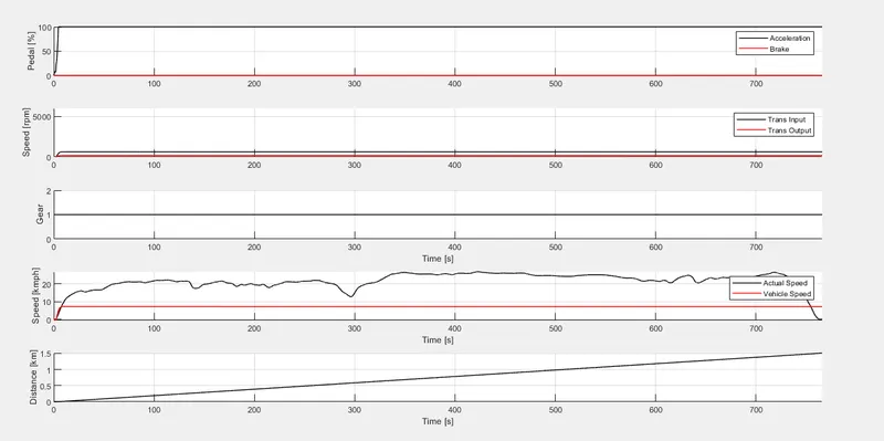
• HWEFT cycle has desired velocity in even manner and the change in controls, outputs differs in increasing.
• Accelerator and brake Pedal percentage with respect to time trace is plotted below in subplot 1. Accelerator pedal is increasing linearly at less time and also the brake pedal is applied at some point only not at high percentage. But the pedal percentage is not so varying at highway and thus the graph appears as flat line.
• The transmission input and output speed is flat in graph and appears similar with respect to time trace as referred in subplot 2. The time trace to attain that speed in both input and output is low.
• Gear command is linear as referred in subplot 3.
• Comparing the desired velocity of the UDDS cycle over actual vehicle velocity in subplot 4, it has huge difference as the curve for desired velocity is varying at different speeds. The actual velocity of vehicle is smoothly increasing and decreasing which is not evident as desired velocity.
• Referring to subplot 5, the distance travelled by any vehicle always increases linearly in even manner.

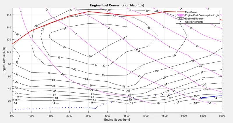
Engine fuel efiiciency map:

• Engine fuel efficiency map is genearted using engine speed in rpm and engine torque in Nm.
• The comtours function is used to create the engine fuel consumption in g/s.
• The map also has maximum torque curve and engine operating points in it.
• The speed of the vehicle ranges from 500 rpm to 6000 rpm.
• The torque generated is ranges from 0 Nm to 170 Nm(approx.)
• The maximum torque curve generates at a speed of 500 rpm and 110 Nm. As well as terminates at speed of 6000 rpm and 150 Nm.
• The maximum torque generated at 165.4 Nm.
• Engine fuel consumption ranges from 1 to 8 g/s. At high speed and high torque, the fuel consumption is also high as 8 g/s.
• The plot has engine efficiency i.e. mileage from 12 to 34%.
• Engine operating condition starts at high speed and zero torque. If we look closely the engine operating condition goes beyond its speed range and the graph line reverses. Engine operating condition is linear upto a point, torque increases linearly and decreases before the speed range.

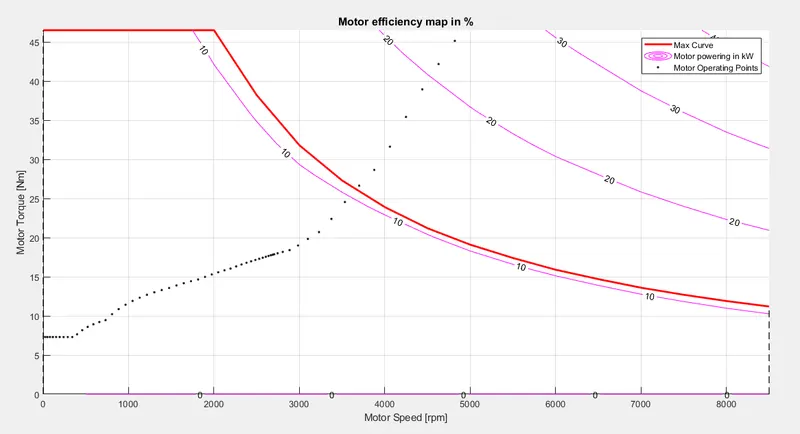
Motor powering map:

• Motor powering map is genearted using motor speed in rpm and motor torque in Nm.
• The contour function is used to create the motor powering map.
• The map also has maximum torque curve and motor operating points in it.
• The speed of the motor ranges from 500 rpm to 8500 rpm.
• The torque generated is ranges from 0 Nm to 61.8 Nm(approx.)
• The maximum torque curve generates at a speed of 500 rpm and 61.8 Nm. As well as terminates at speed of 8500 rpm and 11.2 Nm.
• The maximum torque generated at 61.8 Nm.
• Motor powering ranges from 10 to 40 kW. At high speed and low torque, the power consumption is also high as 40 kW.
• Negative power is plotted which indicates regenerative power from braking of 10 to 20 kW.
• Motor operating condition starts at low speed and low torque. If we look closely the motor operating condition is not frequently operates at speed range and the graph line steeply increases upto torque of 61.8 Nm and speed of 6263 rpm. The motor delivers high torque and high speed at which the transmission delivers a minmum of it due to torque conversion in crank hub.

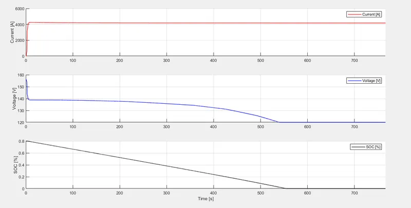
Battery stats:

• Battery delivers power to the hybrid system with terminal voltage and current,
• Battery capacity is measured by state of charge in percentage.
• Time trace of current is 4.242 mA at 8.4 sec and steadily maintains at 4 mA to rest of the cycle.
• Time trace of voltage is 156 V at 0.36 sec and decreases steeply to 138.9 V.
• After which the voltage slowly reaches to 120 V and maintains it till the end of cycle.
• Time trace of SOC is 80% at start and decreases to 0 at 577 sec.

Fuel economy:

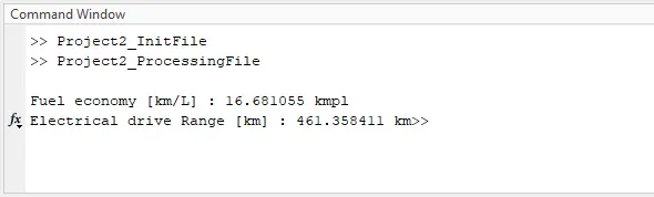
From the workspace, we can see the fuel economy of vehicle for UDDS cyce is 16.681055 kmpl and the range of EV is 461.358411 km.

Conclusion:

UDDS cycle

• Due to more starts/stops in urban drive, the accelerator, brake pedal, gear command is frequently used and speed of the vehicle alters quickly too.
• The engine operating condition is non-linear. It also the engine idling condition, frequent gear shifts imposes more operating points at specific time.
• The motor operating condition is increasing and has more points at start/stops.
• The motor generates high torque initially and generates high speed at the end.
• The fuel economy of vehicle is 16.73 kmpl which is high comparing HWEFT cycle.
• The urban drive has frequent idling condition but the fuel consumption is low due to distance travelled within urban.
• The EV range of vehicle is 259 km which is low comparing HWEFT cycle.
• When motor starts it generates high torque and lowers in high speed.
• The regenrative braking doesn't work properly in intermidiate states.
• So as to know that there is low range on EV due to following reasons,

1. Frequent starts/stops
2. Low regen braking
3. Motor operates at high torque during initial stage
4. The power consumption is high.

HWEFT cycle

• Due to steady drive in highway drive, the accelerator, brake pedal, gear command is not so frequently used and speed of the vehicle stable comparing UDDS cycle.
• The engine operating condition is non-linear. But It has stable engine operating condition, limited gear shifts imposes operating points with time gap.
• The motor operating condition is increasing and less contact with operating points.
• The motor generates high torque initially and generates high speed at the end.
• The fuel economy of vehicle is 16.68 kmpl which is low comparing UDDS cycle.
• The highway drive has frequent driving condition and the fuel consumption is high due to long distance travel in highways.
• The EV range of vehicle is 461 km which is high comparing UDDS cycle.
• When motor starts it generates high torque and lowers in high speed.
• The regenrative braking works properly in these steady states.
• So as to know that there is high range on EV due to following reasons,
• Stable drive condition
• High regen braking
• Motor operates at stable condition so as to perform clear motor operating.
• The power consumption may be high but the regen power restores the battery capcity.

Finally the fuel consumption is nearly same on both cycles but the vehicle performs steadily on HWEFT cycle in EV drive with differences of halfway of UDDS cycle.