Project 2 - Rankine cycle Simulator

AIM: To create a program for Rankine Cycle Simulator and plot T-S, H-S diagram.

OBJECTIVE:

1. Create a Rankine Cycle Simulator.
2. Program a code to calculate the state points of the Rankine Cycle based on user inputs.
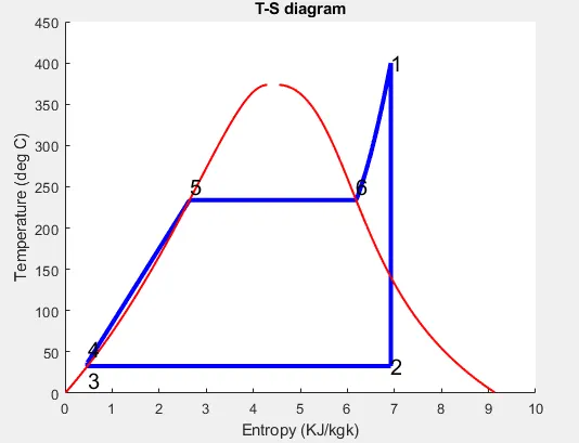
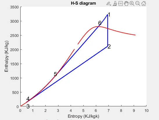
3. Plot the corresponding T-s and h-s diagram for the given set of inputs.

THEORY OF RANKINE CYCLE:

The Rankine cycle is an idealized thermodynamic cylce describing the process by which certain heat engines, such as steam turbines or reciprocating steam engines, allow mechanical work to be extracted from a fluid as it moves between a heat source and heat sink.

Heat energy is supplied to the system via a boiler where the working fluid (typically water) is converted to a high pressure gaseous state (steam) in order to turn a turbine. After passing over the turbine the fluid is allowed to condense back into a liquid state as waste heat energy is rejected before being returned to boiler, completing the cycle.

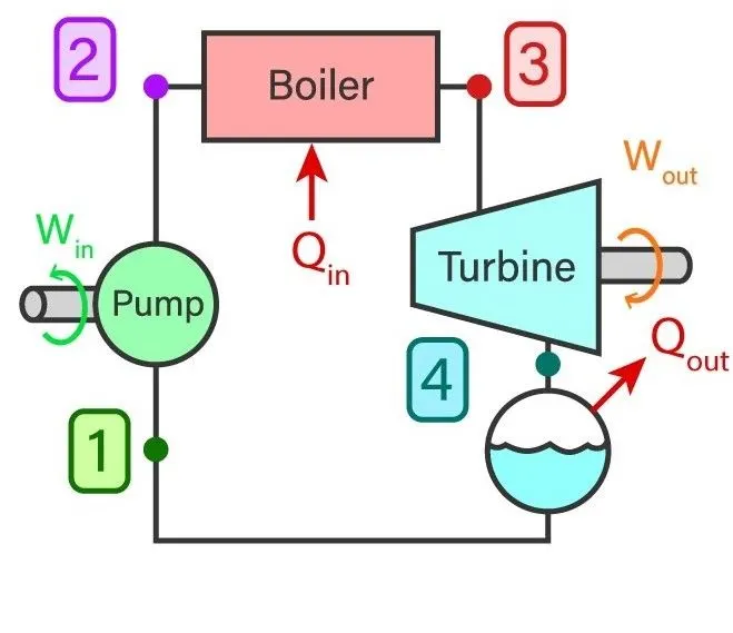
where,

Win - Work done by pump to increase pressure of working liquid.

Wout - output Work given by turbine through rotating shaft where the dry saturated vapor expands.

Qin - Heat produced by boiler high pressure fluid at constant pressure.

Qout - Heat given out by condenser to condense wet vapour to saturated liquid at constant pressure.

PROCESS IN RANKINE CYCLE:

• 1-2: Isentropic compression in pump. Here working fluid is pumped from low pressure to high pressure.
• 2-3: Constant pressure heat addition in the boiler. In this process, the high-pressure liquid is added to the boiler and is heated at constant pressure to become a dry saturated vapour.
• 3-4: Isentropic expansion in a turbine. The dry saturated vapour expands through the turbine resulting in the generation of power.
• 4-1: Constant pressure heat rejection in a condenser. Wet vapour is condensed at a constant pressure to become a saturated liquid.

PROCEDURE:

• Starting a program in MATLAB with the following commands :

1. clear all - To clear all datas stored in workspace.
2. close all - To close previous figures and plots.
3. clc - To clear the command window.

• Then the XSteam.m library is used to get steam table data for water. It is used to calculate the state variable points.
• The given inputs should be entered by the user as,

1. Turbine Inlet temperature = 400° C
2. Turbine Inlet Pressure = 30 bars
3. Turbine Outlet Pressure = 0.05 bars.

• Then to enter the given inputs, we have command p1,t1,p2 are inputs which will be entered by the user.
• If-else command is used to determine the temperature at state one (t1) is greater than normal temperatuer (t) or else the it terminates the iteration by displaying temperature (t) is greater than or equal to saturation temperature .
• So the input variables are taken from Xsteam library by representing respective variable name say Tsat_p is saturation temperature at constant pressure.
• The rest of inputs and its derivatives are entered which is similar to the given code snippet.
• Then enter the derivatives for net work done,efficiency,steam rate per second,work done by pump and work given out by turbine.
• The outputs are shown only by using 'fprintf' command with name of data and its key name where \n is next line, %4.2f is spacing and number after decimal, number of decimals to display.
• To display the vapour line, enter the input by linspace and use for-loop command to generate the h-s value from the code to graph.
• Using 'plot' command, we can derive the H-S diagram for all states of point variables.
• Use concatenation operator, to plot the constant volume varibles.
• Also we can type required 'marker', using marker command.
• By using 'axis' command and enter the required axis value.
• Then name the x-axis as h using 'xlabel' command and y-axis as s using 'ylabel' command.
• Enter the title of the graph using 'title' command.
• The text command displays the number for the respective state point say for s1,h1 point '1' is displayed with respect to the alignment command and its position.
• After the program execution enter the given values for given variables.

ERRORS AND RECTIFICATION:

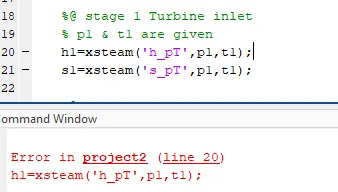
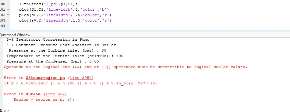
• First I entered incorrect name for the library file as xsteam which is captilized in XSteam. Rectified by replacing the correct name.

• Then I faced the error as the T-S diagram respresented as this. It is a wrong plot there will be a complete plot, vapour line and there is no text representation of state varianble.

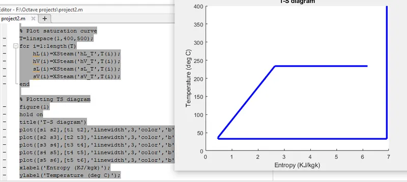
• The vapour line variables should be used in cell array or it should incoprates the logical operators but the vapour line won't displayed. By usind for-loop command it takes number of iterations to fit the cellular arrray and ideal vapour line will be displayed.

PROGRAM:

clear all
close all
clc

% Theory of rankine cycle
fprintf('    RANKINE CYCLE SIMULATOR     \n ');
fprintf('1-2 Isentropic Expansion in Turbine\n ');
fprintf('2-3 Constant Pressure Heat Rejection in Condenser\n ');
fprintf('3-4 Isentropic Compression in Pump\n ');
fprintf('4-1 Constant Pressure Heat Addition in Boiler\n ');

% inputs
p1=input(' Pressure at the Turbine inlet (bar) : ');
t1=input(' Temperature at the Turbine inlet (celsius) : ');
p2=input(' Pressure at the Condenser (bar) : ');

%@ stage 1 Turbine inlet
% p1 & t1 are given
h1=XSteam('h_pT',p1,t1);
s1=XSteam('s_pT',p1,t1);

%@ stage 2 Condenser inlet
% p2 is given
s2=s1;
sf2=XSteam('sL_p',p2);
sg2=XSteam('sV_p',p2);
hf2=XSteam('hL_p',p2);
hg2=XSteam('hV_p',p2);
x2=(s2-sf2)/(sg2-sf2);
h2=hf2+(x2*(hg2-hf2));

%@ stage 3 Pump inlet
p3=p2;
h3=XSteam('hL_p',p3);
s3=XSteam('sL_p',p3);
t3=XSteam('Tsat_p',p3);
t2=t3;

%@ stage 4 Boiler inlet
p4=p1;
s4=s3;
h4=XSteam('h_ps',p4,s4);

Cp4=XSteam('Cp_ps',p4,s4);
Cv4=XSteam('Cv_ps',p4,s4);
lambda=Cp4/Cv4;
t4=t3/((p3/p4)^((lambda-1)/lambda));

t5=XSteam('Tsat_p',p1);
t6=t5;
s5=XSteam('sL_p',p1);
s6=XSteam('sV_p',p1);
h5=XSteam('hL_p',p1);
h6=XSteam('hV_p',p1);

% Turbine work
wt=h1-h2;

% Pump work
wp=h4-h3;

% Net work (KJ/kg)
w=wt-wp;

% Heat in & out of the system
Q_in=h1-h4;
Q_out=h2-h3;

% Thermal efficiency
Efficiency=(w/Q_in)*100;

% Steam rate (kg/kwh)
ssc=3600/w;

% Back work ratio
BWR=(h1-h4)/(h2-h3);

% Plot saturation curve
T=linspace(1,400,500);
for i=1:length(T)
    hL(i)=XSteam('hL_T',T(i));
    hV(i)=XSteam('hV_T',T(i));
    sL(i)=XSteam('sL_T',T(i));
    sV(i)=XSteam('sV_T',T(i));
end

% Plotting TS diagram
figure(1)
hold on
title('T-S diagram')
plot([s1 s2],[t1 t2],'linewidth',3,'color','b')
plot([s2 s3],[t2 t3],'linewidth',3,'color','b')
plot([s3 s4],[t3 t4],'linewidth',3,'color','b')
plot([s4 s5],[t4 t5],'linewidth',3,'color','b')
plot([s5 s6],[t5 t6],'linewidth',3,'color','b')
xlabel('Entropy (KJ/kgk)');
ylabel('Temperature (deg C)');
S1=linspace(s6,s1,500);
for j=1:length(S1);
    T1(j)=XSteam('T_ps',p1,S1(j));
end
plot(S1,T1,'linewidth',3,'color','b')
plot(sL,T,'linewidth',1.5,'color','r')
plot(sV,T,'linewidth',1.5,'color','r')

% Annotations
text(s1,t1,'1','fontsize',15);
text(s2,t2,'2','fontsize',15);
text(s3,t3,'3','fontsize',15,'verticalalignment','top');
text(s4,t4,'4','fontsize',15,'verticalalignment','bottom');
text(s5,t5,'5','fontsize',15,'verticalalignment','bottom');
text(s6,t6,'6','fontsize',15,'verticalalignment','bottom');

% Plotting H-S diagram
figure(2)
hold on
title('H-S diagram')
plot([s1 s2],[h1 h2],'linewidth',2,'color','b')
plot([s2 s3],[h2 h3],'linewidth',2,'color','b')
plot([s3 s4],[h3 h4],'linewidth',2,'color','b')
xlabel('Entropy (KJ/kgk)');
ylabel('Enthalpy (KJ/kg)');
H4=linspace(h4,h5,500);
for k=1:length(H4);
    S4(k)=XSteam('s_ph',p1,H4(k));
end
H6=linspace(h6,h1,500);
for m=1:length(H6);
    S6(m)=XSteam('s_ph',p1,H6(m));
end
plot(S4,H4,'linewidth',2,'color','b')
plot([s5 s6],[h5 h6],'linewidth',2,'color','b')
plot(S6,H6,'linewidth',2,'color','b')
plot(sL,hL,'linewidth',1.5,'color','r')
plot(sV,hV,'linewidth',1.5,'color','r')

% Annotations
text(s1,h1,'1','fontsize',15);
text(s2,h2,'2','fontsize',15);
text(s3,h3,'3','fontsize',15,'verticalalignment','top');
text(s4,h4,'4','fontsize',15,'verticalalignment','bottom');
text(s5,h5,'5','fontsize',15,'verticalalignment','bottom');
text(s6,h6,'6','fontsize',15,'verticalalignment','bottom');

% Result window
fprintf('\nRESULTS\n');
fprintf('\nAt state point 1 :\n');
fprintf('P1=%f Bar\n',p1);
fprintf('T1=%f Deg Celsius\n',t1);
fprintf('H1=%f KJ/kg\n',h1);
fprintf('S1=%f KJ/kgk\n',s1);

fprintf('\nAt state point 2 :\n');
fprintf('P2=%f Bar\n',p2);
fprintf('T2=%f Deg Celsius\n',t2);
fprintf('H2=%f KJ/kg\n',h2);
fprintf('S2=%f KJ/kgk\n',s2);

fprintf('\nAt state point 3 :\n');
fprintf('P3=%f Bar\n',p3);
fprintf('T3=%f Deg Celsius\n',t3);
fprintf('H3=%f KJ/kg\n',h3);
fprintf('S3=%f KJ/kgk\n',s3);

fprintf('\nAt state point 4 :\n');
fprintf('P4=%f Bar\n',p4);
fprintf('T4=%f Deg Celsius\n',t4);
fprintf('H4=%f KJ/kg\n',h4);
fprintf('S4=%f KJ/kgk\n',s4);

fprintf('\nWork done by Turbine is : %f KJ/kg\n',wt);
fprintf('Work done by Pump is : %f KJ/kg\n',wp);
fprintf('Net work done on the system : %f KJ/kg\n',w);
fprintf('Specific steam consumption is : %f kg/KWh\n',ssc);
fprintf('The Net thermal efficiency of the system is : %f\n',Efficiency);
fprintf('The BWR of the rankine cycle is found to be : %f\n',BWR);

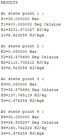
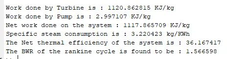
OUTPUTS:

PLOT: