Week 4.1 - Genetic Algorithm

AIM: Write a program to optimise the genetic algorithm using MATLAB.

OBJECTIVE:

1. A program to optimise the stalagmite function and find the 'global maxima' of the function.
2. To expalin the concept of genetic algorithm and also explain the syntax for 'ga' in MATLAB.
3. Plot graphs for 3 optimization studies as follows,

• With un-constrained inputs.
• With constrained lower and upper bounds.
• With constrained inputs and increased population size.

PROCEDURE:

[1] To optimise the stalagmite function and find the 'global maxima' of the function

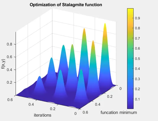
• Stalagmite is a type of rock formation in caves as the upside down triangles accumalating the depostions from ceiling to floor as shown in plot section.
• Start the program by creating a stalagmite function in separate file.
• Enter the input vectors x and y.
• Then enter the stalagmite model derivation is as follows.

- f(x,y) = f1x* f1y* f2x* f2y

- f1x (f1) = sin(5.1*pi*x+0.5)^6

- f1y (f2) = sin(5.1*pi*y+0.5)^6

- f2x (f3) = exp(-4*log(2)*(x-0.0667)^2/0.64)

- f2y (f4) = exp(-4*log(2)*(y-0.0667)^2/0.64)

• As the function output is 'f', determine it as f(x,y) derivative with negative sign as it indiactes the maxima function.
• First optimise the stalagmite function and then find the global maxima function.
• We defined the input vectors in function file but determining its value using linspace command fulfills the function.
• Using linspace command, it generates the numbers from starting number to end number along with the total numbers to be displayed.
• It is used as follows linspace(x,y,z).
• where, x= staring value of velocity.
• y= ending value of velocity.
• Then defining the population size using num_cases as it finds only the optimal number of iterations for ga.
• Then use tic-toc command to calculate the time of evaluating the code.
• Meshgrid defines the input variable in two dimensional array.
• Use for-loop to determine the controlled form of structure to execute it in given iterations.
• Now define the stalagmite function in the program.
• As we going to get different plots, So use figure command to separate different plots.
• Use the surfc command to get a surface plot as output. Since it is a 3D plot we have to define the input and output varibles as well.
• Using 'plot' command, we can derive the graph for velocity and drag force. Also we can type required 'color', 'marker', 'linewidth' usign respective commands.
• By using 'axis' command and enter the required axis value.
• Then name the x-axis using 'xlabel' command and y-axis using 'ylabel' command.
• Enter the title of the graph using 'title' command
• Use 'grid' command to enable grids in graph.

[2] Genetic algorithm

• Genetic algorithm (ga) is an evolutionary algorithms which uses darwin's theory survival of the fittest to get optimal solution.
• It selesct the individuals from random of the population on mate and produces outputs.
• The ouputs must mutate in every genration and provide an optimal solutions.
• It can be used to any optimization problems that are non-linear, non-differential and discontinuos.
• Syntax for genetic algorithm,

[x,fval,exit,output,population,fvalue] = ga(func,n,A,B,[],[],lb,ub,nlncon,intcon,options)

where,

x = Local minimum

fval = Fitness value

exit = Reason ga stopped

output = Output for each generations

population = Final popualtion

fvalue = Final score

ga = Genetic algorithm command

func = Objective function

n = Number of variables

A,B,[],[] = Linear inequalities as A*x<=B

lb = Lower bound

ub = Upper bound

nlncon = Non-linear constraints which accepts the vector arrays.

intcon = integer variables

options = Optimization option

CODE:

function f = stalagmite(input_vector)
x=input_vector(1);      % input variable 1
y=input_vector(2);      % input variable 2
f1=(sin(5.1*pi*x+0.5))^6;
f2=(sin(5.1*pi*y+0.5))^6;
f3=exp(-4*log(2)*(x-0.0667)^2/0.64);
f4=exp(-4*log(2)*(y-0.0667)^2/0.64);
f=-(f1*f2*f3*f4);       % negative sign indicates the maxima function
end

% A prorgram to run stalagmite mathematical model
%input variables
x=linspace(0,0.6,150);
y=linspace(0,0.6,150);
num_cases=50
% create two dimensional array
[x,y]=meshgrid(x,y);

% Evaluate the stalagmite function
func=zeros;
for i=1:length(x)
    for j=1:length(y)
        input_vector(1)=x(i,j);
        input_vector(2)=y(i,j);
        func(i,j)=stalagmite(input_vector);
    end
end

%plotting
figure (1)
surfc(x,y,-func)
xlabel('iterations')
ylabel('funcation minimum')
zlabel('f(x,y)')
title('Optimization of Stalagmite function')
shading interp

% study 1 unbounded optimization
tic
objfunc=@stalagmite;
for i=1:num_cases
    [inputs,fopt(i)]=ga(objfunc,2);
    xopt(i)=inputs(1);
    yopt(i)=inputs(2);
    end
time=toc

%plotting
figure(2)
subplot(2,1,1)

surfc(x,y,-f)
shading interp
plot3(xopt,yopt,-fopt,'marker','x','markersize',5,'markerfacecolor','r')
hold on
title('unbounded inputs')
subplot(2,1,2)
plot(fopt)
xlabel('iterations')
ylabel('funcation minimum')

% study 2 with upper and lower bounds
tic
for i=1:num_cases
    [inputs,fopt(i)]=ga(@stalagmite,2,[],[],[],[],[0;0],[1;1]);
    xopt(i)=inputs(1);
    yopt(i)=inputs(2);
    end
time=toc

%plotting
figure(3)
subplot(2,1,1)
hold on
surfc(x,y,-f)
shading interp
plot3(xopt,yopt,-fopt,'marker','x','markersize',5,'markerfacecolor','r')
title('Constained upper and lower bounds')
subplot(2,1,2)
plot(-fopt)
xlabel('iterations')
ylabel('funcation minimum')

% study 3 increasing ga increases
options=optimoptions('ga');
options=optimoptions(options,'populationsize',170);
tic
for i=1:num_cases
    [inputs,fopt(i)]=ga(@stalagmite,2,[],[],[],[],[0;0],[1;1],[],[],options);
    xopt(i)=inputs(1);
    yopt(i)=inputs(2);
    end
time=toc

%plotting
figure(4)
subplot(2,1,1)
hold on
surfc(x,y,-f)
shading interp
plot3(xopt,yopt,-fopt,'marker','x','markersize',5,'markerfacecolor','r')
title('Constrained inputs and increased population size')
subplot(2,1,2)
plot(fopt)
xlabel('iterations')
ylabel('funcation minimum')

ERRORS:

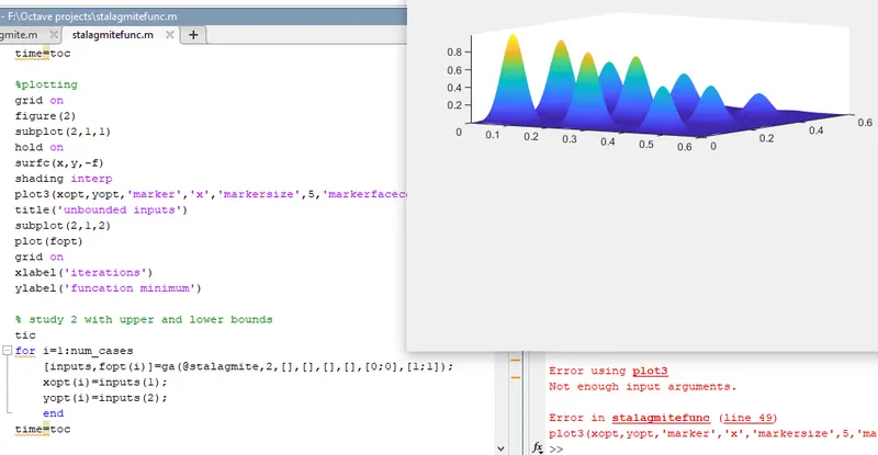
• Only one error I faced is without ploting the output 'fopt' in plotting. So it generates an error as not enough input arguments.
• Since generates stalagmite model but the output function doesn't form as in plot section.

PLOT:

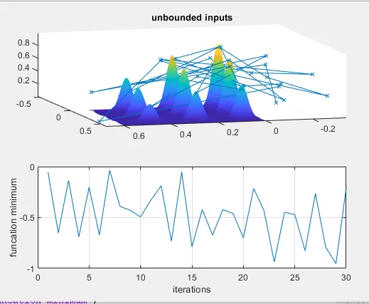
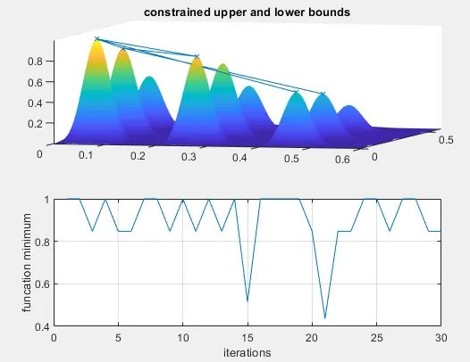
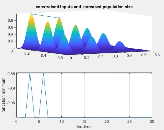
• Number of iterations = 30
• Time taken to optimise the unconstrained inputs.= 2.284 seconds.
• Time taken to optimise the constrained lower and upper bounds = 2.831 seconds.
• Time taken to optimise the constrained inputs and increased population size = 5.940 seconds.
• MAXIMA of stalagmite function optimized in unconstrained inputs.= 0.977
• MAXIMA of stalagmite function optimized in constrained lower and upper bounds = 1
• MAXIMA of stalagmite function optimized in constrained inputs and increased population size = 1
• The stalagmite function lies at x=0.06 and y=0.03.

CONCLUSION:

We get the genetic algorithm to optimize the stalamite fucntion and the optimal global maxima value is 1 which lies at x=0.06 and y= 0.03.

REFERENCES:

• Genetic algorithm optimization by alexander robbles.
• Genetic algorithm by c.balaji