Project 2

THEORY:

Forward-Modelling Approach:

• The engine-to-wheel, rear-to-front, and cause-and-effect methods are other names for the forward modelling methodology. Calculation flows in the same direction as positive power flow from engine to wheel.
• This method is based on equations for vehicle dynamics, the behaviour of individual powertrain parts, and their dynamic interplay.
• A driver controller is also needed to set the calculations' start time and regulate the car to follow a desired speed. In order to investigate driver behaviour, the controller is set up to model how the driver will operate the brakes or the accelerator to match the intended speed. A feedback loop that the controller is a part of will be utilised to calculate how much energy is needed to move the vehicle.

P1 Hybrid:

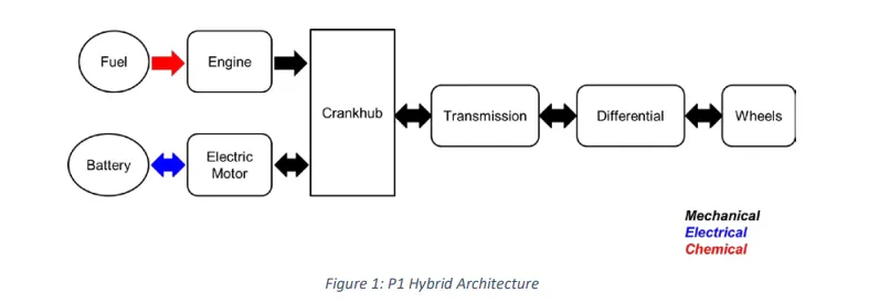
For this project, a Honda Insight motor and battery are under consideration. The information is derived from the NREL, USA-developed ADVISOR data base. There is data in the project files. 

VEHICLE MODEL:

Pre-Processing:

• All the variables required to run and post-process the Simulink model have been loaded using a MATLAB script. From here, you may also choose the drive cycle. The script is initialised in MATLAB to load all the workspace variables before the Simulink vehicle model is run.

%%%%%%%%%%%%%%%%%%%%%%%%%%%%%%%%%%%%%%%%%%%%%%%%%%%%%%%%%%%%%%%%%%%%%
%% Skill-Lync -> Hybrid Drives Development
% Project 1 - Conventional Vehicle Model
% By - Ullekh Gambhira 

% Description:

%% Initialization File
% Initialization file for loading the variables for the Conventional vehicle simulation model

%% Vehicle Parameters
M = 1500;       % Vehicle weight [kg]
Cr = 0.015;     % Rolling resistance coefficient
Rw = 0.35;      % Rolling radius [m]
Cd = 0.33;      % Drag coefficient
Af = 2;         % Frontal area [m2]
rhoa = 1.225;   % Air density [kg/m3]
Vwind = 0;      % Wind velocity [kmph]
g = 9.81;       % Gravitational acceleration [m/s2]
theta = 0;      % Slope [deg]
myu_road_tire = 1; % Coefficient of friction between tire - road interface

%% Powertrain Parameters 
FDR = 3.73;                         % Final Drive Ratio / Diff Ratio
DiffEff = 0.99;                     % Differential efficiency (assumed independent of operating conditions)

NumGear = 4;                        % Number of gears in transmission
TransGear = [1:NumGear];            % Transmission Gears
TransRatio = [3.06, 1.62, 1, 0.7];  % Corresponding Transmission ratios
TransEff = 0.90;                    % Transmission efficiency (assumed independent of operating conditions)

TC_SR = [0, .5, .6, .7, .8, .87, .92, .94, .96, .97, 1];   % Torque Converter Speed Ratio (Matlab default) -> TurbSpd/PumpSpd  
TC_TR = [2.232, 1.5462, 1.4058, 1.2746, 1.1528, 1.0732, 1.0192, 1, 1, 1, 1];   % Torque Converter Torque Ratio (Matlab default) -> TurbTrq/PumpTrq
TC_Cf = 1e-4 * [.72558, .66322, .63463, .59042, .51331, .4144, .29287, .22444, .12186, .04386, 0]; % Torque Converter Capacity Factor (Matlab default) -> PumpTrq/PumpSpd^2 [Nm/rpm^2]

load Vehicle_Data/Engine_data_1_9L_Saturn_95kW
load Vehicle_Data/Trans_Shift_map
load Vehicle_Data/EM_Honda_Insight_10kW
load Vehicle_Data/ESS_NiMH6


ESS_init_soc = 0.8;
ESS_soc_max = 0.9;
ESS_soc_min = 0.6;


%% Driver Parameters
Kp = 10;                    % P gain for driver PI model
Ki = 1;                     % I gain for driver PI model
Drive_Cycle_Select = 2;     % Drive cycle selection

% Drive cycle values in m/s

if Drive_Cycle_Select == 1
    load DriveCycles/UDDS;
    
elseif Drive_Cycle_Select == 2
    load DriveCycles/HWFET;
    
elseif Drive_Cycle_Select == 3
    load DriveCycles/FTP;
    
elseif Drive_Cycle_Select == 4
    load DriveCycles/US06;
    
elseif Drive_Cycle_Select == 5
    load DriveCycles/NEDC;
    
elseif Drive_Cycle_Select == 6
    load DriveCycles/WLTP;
 
end

time_end = cyc_time(end);
vel_end = cyc_vel(end);

• The Drive Cycle can be selected from this MATLAB Script, By changing the variable Drive _Cycle _Select to,

1. UDDS
2. HWFET
3. FTP
4. USO6
5. NEDC
6. WLTP

SIMULINK MODELLING:

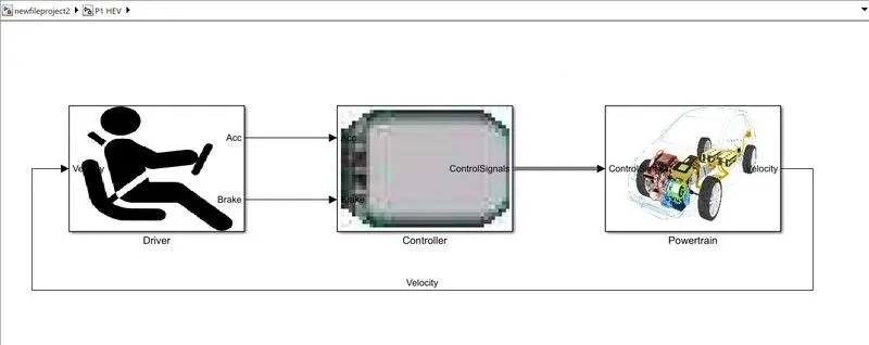
• Three primary sub-blocks for the driver model, control model, and powertrain block are used to produce the Simulink model for the convection model.
• The driver block receives feedback on the real vehicle speed, and the driver block transmits to the controller block the necessary output for accelerating or braking. The controller block then sends control signals to the powertrain model for engine torque, gear shifting, and brake torque.

Driver Model :

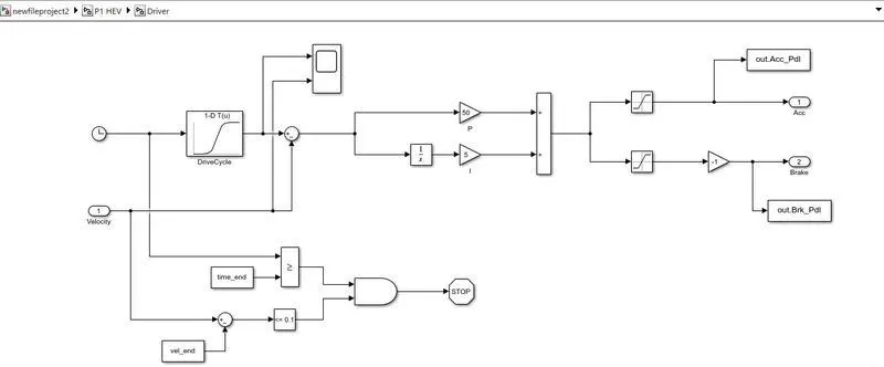
A fundamental PI controller called Driver Model produces outputs from the accelerator and brake pedals that are matched to the desired and actual vehicle speeds.

By giving the controller output for the accelerator and brake pedals, the PI controller manages the discrepancy between the needed driving cycle and the actual vehicle speed.

Controller Model :

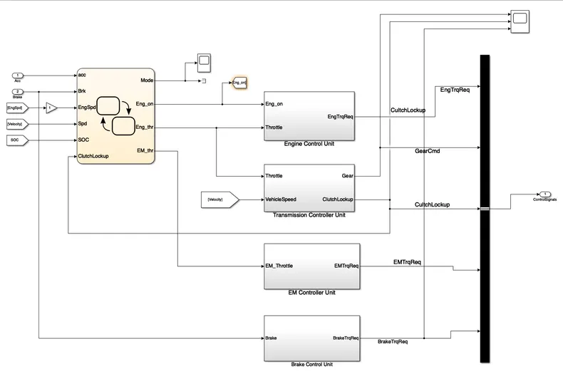
• As a representation of the electronic control components, the "Controller block" serves as the vehicle's brain. It produces the required engine torque, desired motor torque, desired transmission gear, and desired brake torque based on inputs from the driver. These inputs are supplied to the block labelled "Powertrain," which symbolises the vehicle's drivetrain.
• The supervisory control unit, which chooses between start/stop, cruise, and regeneration braking modes, is represented by a state flow machine. The controller is in charge of managing the motor and engine drives for each mode.

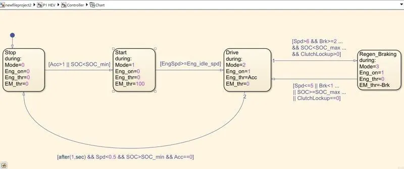
• The accelerator and brake pedal inputs from the driver unit, the engine's actual speed, the vehicle's actual speed, the SOC status, and the clutch lockup state are the inputs to the state flow charts. Moreover, the mode, engine on/off request, engine input throttle, and electric motor input throttle are the state flow outputs to the various controllers.
• An electric motor control unit, a transmission control unit, an engine control unit, and a brake control unit make up the controller.
• All control signals are again passed to the transmission model, which represents the drive train. 

Engine Control Unit :

 

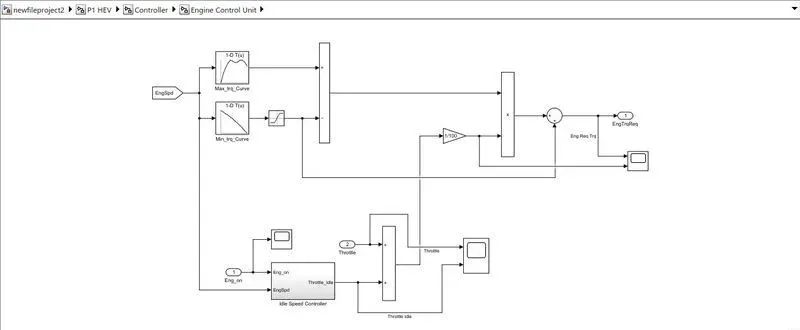
We use an engine control unit in this control model, which provides input for the engine speed by building a look-up table. We feed maximum torque and map speed into that table, and we also establish a second look-up table in which we input CT torque and map speed, from which it subtracts and multiplies. The engine speed also provides the appropriate control speed, which we may incorporate to produce the engine's reqired torque.

Electric Motor Control Unit:

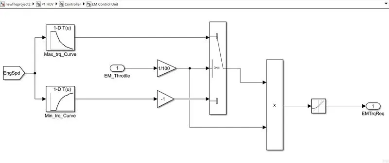
The motor control unit Give the electric motor the necessary torque command by comparing its speed with the lookup table's maximum torque and maximum torque generation curves. Comparing the lookup tables and calculating the torque input needed for the E-Motor both use the EM throttle input.

Transmission Control Block:

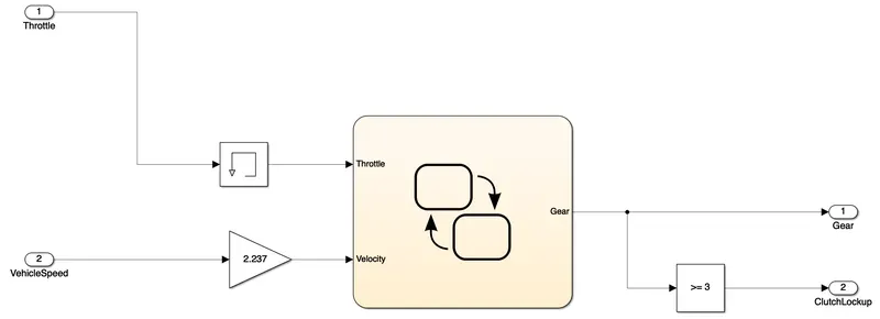
The transmission control block controls the gear shifting using the study flow Varianble chart.

Brake Control Unit:

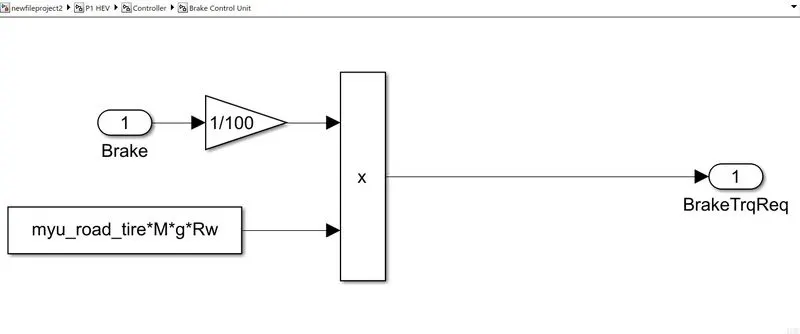
In this calculate brake torque and then all three control signals output is give to powertrain.

Powertrain Model :

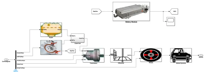
All the parts that transform an engine's power into motion are included in the powertrain model.

This covers the subsystems for the vehicle's body dynamics as well as the engine, battery pack, electric motor, crank hub, transmission, differential, wheels, and wheels.

The appropriate blocks in the powertrain model get the control signals from the control model through a bus.

Battery Model:

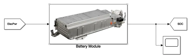
With electric power as the input and battery SOC as the output, a battery pack subsystem is produced.

The SOC and terminal voltage are each determined by a different sub-block, with the terminal voltage being calculated using the SOC.

SOC Estimation Model:

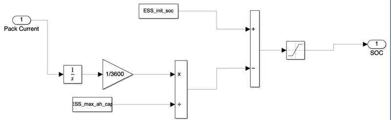
To calculate the SOC of the battery at each instance, the pack current in amps is converted to amp hours, multiplied by the maximum capacity, and added to the initial SOC. The result is limited to a value between 0 and 1.

Terminal Voltage Model:

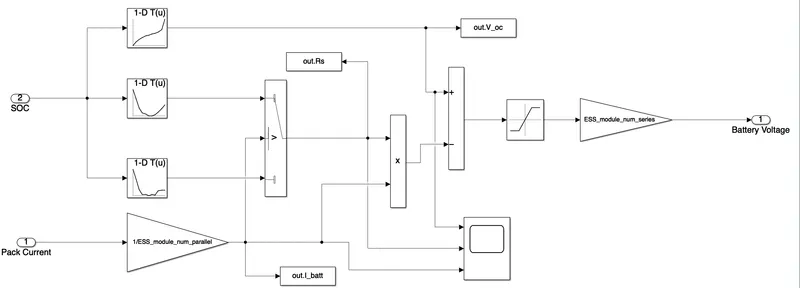
ID lookup tables are used to establish ideal voltage and internal resistance, and the model is used to determine battery voltage.

The Two Workspace block sends the supplied values back to workspace, where they can be utilised for post-processing.

Engine Model:

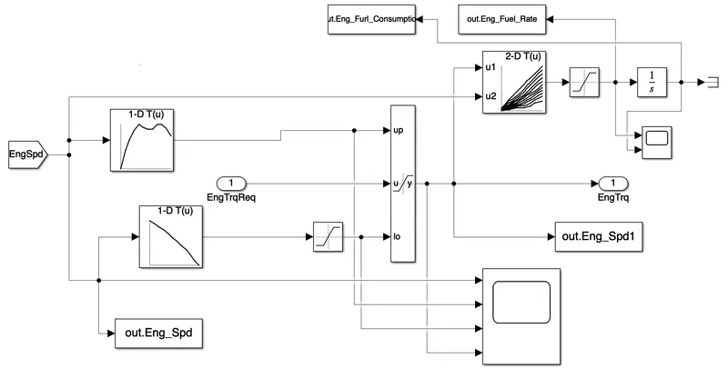
Depending on engine speed The controller's needed torque is saturated between the maximum and minimum torque curves, passing the engine's torque to the transmission block.

Based on engine speed and torque, the fuel flow rate is calculated using a 2D lookup table. The fuel consumption is then calculated using an integration of the fuel flow rate.

The to-workspace block is used to send estimated values for fuel flow rate, fuel consumption, engine torque, and engine speed to the MATLAB workspace.

Fuel usage and engine fuel flow rate are measured.

Electric Motor Model: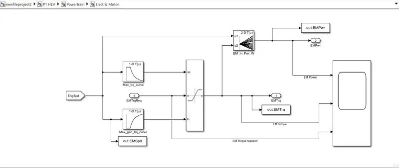

Depending on engine speed Between the maximum EM torque curve and the maximum EM torque generation curve, the controller's necessary EM torque is saturated, which then transmits the EM torque to the crank hub.

Based on EM speed and EM torque, the 2D lookup table is utilised to determine the motor's input electric power.

Crank Hub:

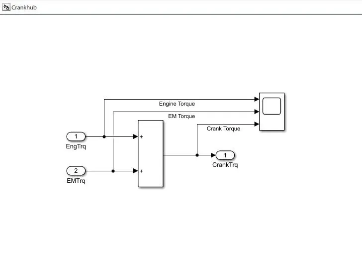
The transmission block receives the crank torque from the crank hub after adding the EM torque and engine torque.

Transmission Model:

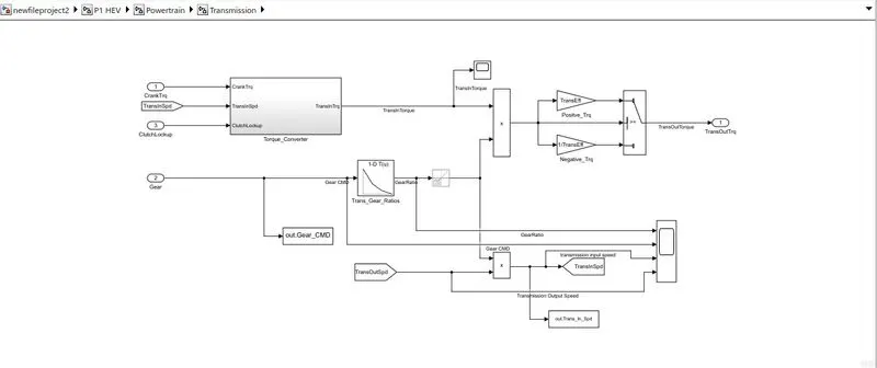
We use the engine torque and the gear selector from the controller to transmit the gear ratio in these models. After multiplying the ratio by the transmission's input torque, positive and negative transmission efficiency torques are used to determine the gearbox's input speed. This torque converter, which is a component of the transmission, connects the engine to the transmission. Engine dynamics are essentially disconnected from it.

Torque Converter:

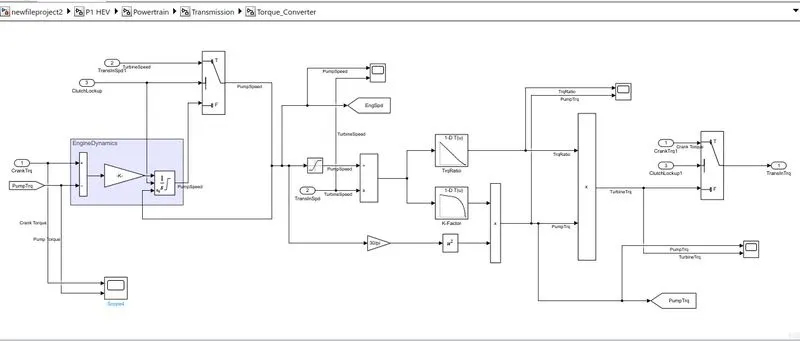
By using the clutch lockup status to determine the pump and turbine torque, the torque converter determines the appropriate transmission torque.

Differential Model: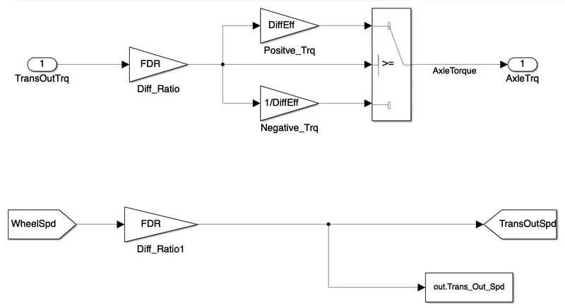

In this block, the differential ratio and differential efficiency are multiplied with the transmission output torque to produce the axle torque, which is then sent to the wheel.

Wheel Model:

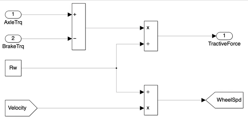
To calculate the tractive force, the axle torque from the control model is subtracted from the brake torque, which is then divided by the rolling radius.
The vehicle velocity is used to calculate the wheel speed, which is then saved in the workspace.

Vehicle Dynamics:

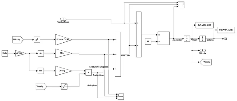
The longitudinal dynamics of the vehicle along with the road load is represented in the 'Vehicle Dynamics' block.

Tractive Force and Road loads are used to calculate the vehicle velocity.

The variables are loaded on the workspace using MATLAB script.

The Acceleration, Velocity and Distance travelled are Calculation and stored in the workspace.

SIMULATION RESULTS

UDDS Drive Cycle :

Drive Cycle and Actual Velocity

Model

Post-Processing:

To analyse data and create charts, a MATLAB script is written. Here, we rename the model-loaded variables, perform some elementary post-processing computations, and provide results and visualisations.

%% Post-Processing File
%  File for post-processing the Conventional vehicle simulation model data


%% Renaming variables
Time = out.tout;
Acc_Pdl = out.Acc_Pdl;          % Accelerator pedal [%]
Brk_Pdl = out.Brk_Pdl;          % Brake pedal [%]
Gear_Cmd = out.Gear_Cmd;        % Transmission gear
Trans_In_Spd = out.Trans_In_Spd*30/pi;  % Transmission input speed [rpm]
Trans_Out_Spd = out.Trans_Out_Spd*30/pi;% Transmission output speed [rpm]
Eng_Trq = out.Eng_Trq;          % Engine brake torque [Nm]
Eng_Spd = out.Eng_Spd*30/pi;    % Engine speed [rpm]
Eng_Fuel_Consump = out.Eng_Fuel_Consumption;    % Engine fuel consumption [g]
Veh_Dist = out.Veh_Dist/1000;   % Distance traveled by vehicle [km]
Veh_Spd = out.Veh_Spd*18/5;     % Vehicle speed [kmph]


%% Data Analysis
Eng_Pwr = Eng_Spd*pi/30.*Eng_Trq/1000;   % Engine brake power [kW]
rho_petrol = 0.7197;                    % Density of petrol [kg/L]
kmpl = Veh_Dist(end)/(Eng_Fuel_Consump(end)/1000/rho_petrol);    % Fuel economy [kmpl] 


%% Plotting vehicle characteristics time trace
figure()
subplot(3,1,1)
hold on
grid on
plot(Time, Acc_Pdl, 'linewidth', 1, 'Color', 'black');
plot(Time, Brk_Pdl, 'linewidth', 1, 'Color', 'red');
ylabel('Pedal [%]')
xlim([0, Time(end)]);
legend('Accel','Brake');
subplot(3,1,2)
hold on
grid on
plot(Time, Trans_In_Spd, 'linewidth', 1, 'Color', 'black');
plot(Time, Trans_Out_Spd, 'linewidth', 1, 'Color', 'red');
ylabel('Speed [rpm]')
xlim([0, Time(end)]);
ylim([0, 6000]);
legend('Trans Input','Trans Output');
subplot(3,1,3)
hold on
grid on
plot(Time, Gear_Cmd, 'linewidth', 1, 'Color', 'black');
xlim([0, Time(end)]);
xlabel('Time [s]');
ylabel('Gear');


%% Plotting engine operating points on engine fuel map
figure('Name','Engine Operating Points');
hold on
grid on
title('Engine Operating Points','fontsize',12);
p1=plot(Eng_map_spd*30/pi,Eng_max_trq,'linewidth',2,'color','r');
p2=line([Eng_map_spd(end)*30/pi Eng_map_spd(end)*30/pi],[0 Eng_max_trq(end)]);
set(p2,'linewidth',1,'linestyle','--','color','k');
p3=line([Eng_map_spd(1)*30/pi Eng_map_spd(1)*30/pi],[0 Eng_max_trq(1)]);
set(p3,'linewidth',1,'linestyle','--','color','k');
[c,h] = contour(Eng_map_spd'*30/pi,Eng_map_trq,Eng_fuel_map');
clabel(c,h);
xlabel('Engine Speed [rpm]');
ylabel('Engine Torque [Nm]');
title('Engine Fuel Consumption Map [g/s]');
p4 = plot(Eng_Spd,Eng_Trq,'.','color','k');
legend([p1 p4],{'Max Curve','Operating Points'});
axis([Eng_map_spd(1)*30/pi Eng_map_spd(end)*30/pi 0 Eng_map_trq(end)]);

Result:

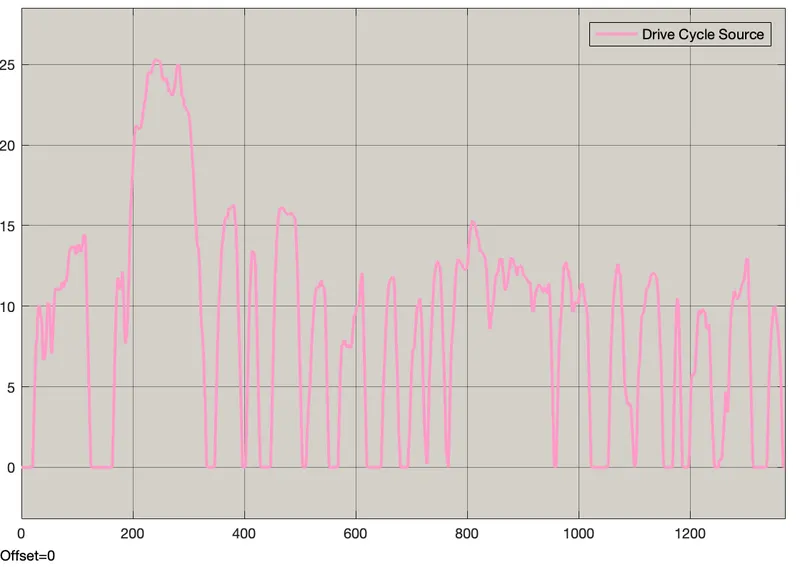
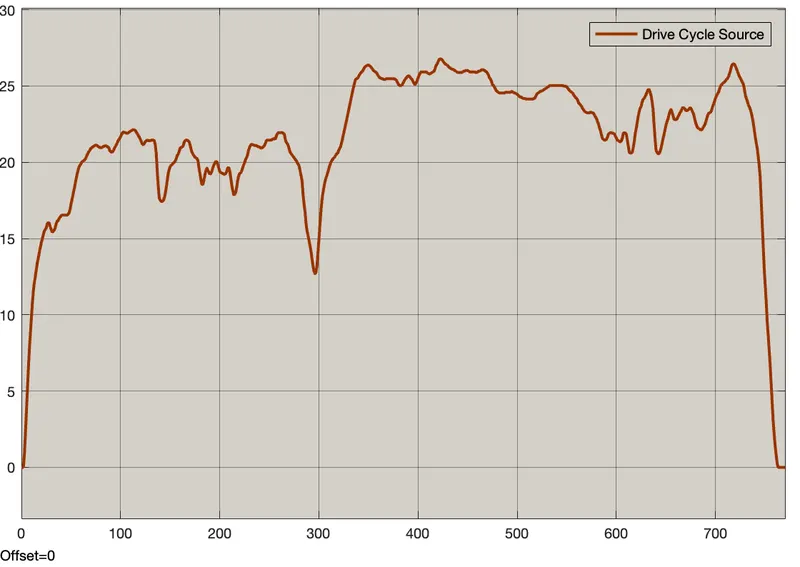
Drive Cycle 

UDDS:

HWFET:

Fuel economy numbers (kmph) for UDDS and HWFET cycle.

UDDS :

Fuel economy improves as engine eliminates negative torque and negative power. Negative Energy can be revived with regional breaking.

 HWFET:

Although there is less negative power on the highway when driving, fuel economy is marginally enhanced. Regen braking, however, will generate all negative power, increasing battery SOC.
Because there is less brake pedal engagement and idle time during the drive cycle, city fuel economy is significantly lower than highway fuel economy.

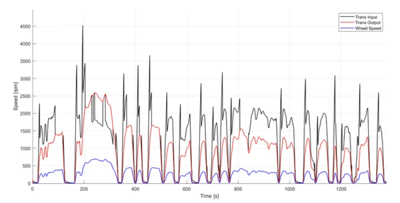
The Time trace for engine, Transmission input,transmission output and wheel speed

UDDS:

 

HWFET:

 

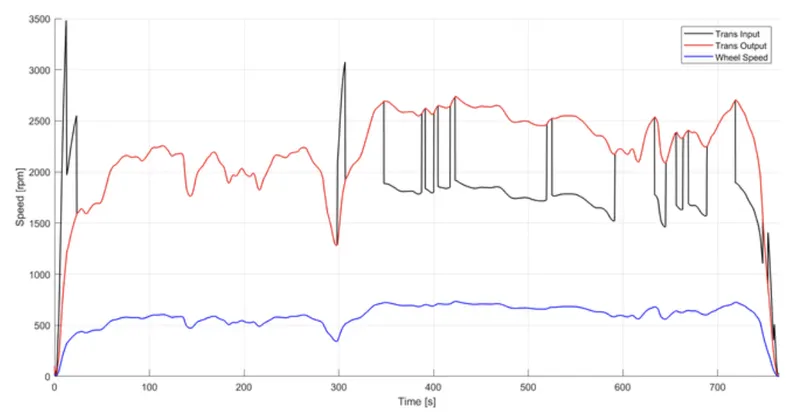
The torque converter contributes significantly to the input speed fluctuation, and the transmission input speed fluctuates in accordance with the engine torque required to complete the driving cycle.

Differential and gear ratios affect wheel speed and transmission output speed.

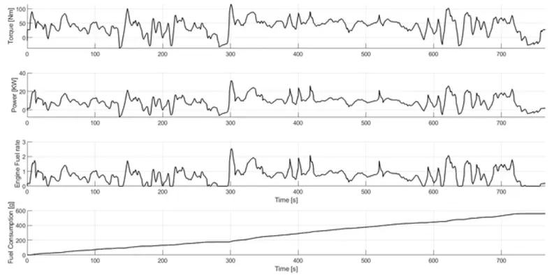
Engine troque, Engine power, fuel rate and fuel consumption

UDDS :

HWFET :

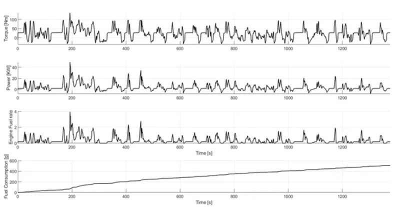
When the drive cycle's torque needs fluctuate, the fuel flow rate also varies, and fuel consumption is estimated.

The HWFET drive cycle requires more positive torque and power and less negative torque and power.

Accelerator and brake pedal, gear command, vehicle desired and actual speed, vehicle distance

UDDS:

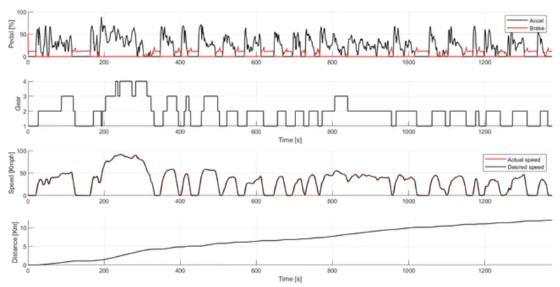
Because the drive cycle is not very smooth and gear shifts are required frequently, the accelerator and brake pedals are utilised more frequently.

HWFET:

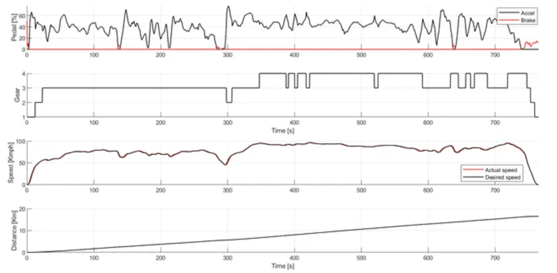
The highway drive cycle is smoother, which reduces the need for stopping and increases the amount of acceleration. It also results in more frequent gear adjustments.

Plots show the needed speed of the vehicle, the real vehicle speed, the actual vehicle distance, the accelerator and brake pedals, and the gear command of the transmission control unit.

The engine operating points on the engine fuel map: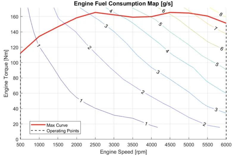

On the fuel map, the engine operating point is shown, and it is below the maximum torque curve.

The Motor speed, torque, motor input power.

UDDS:

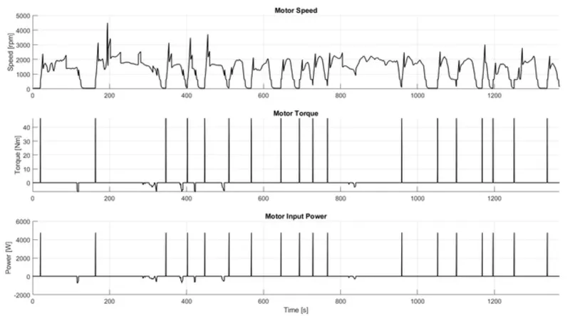
Just the engine start and brake operations require motor torque. The motor speed in relation to the requested EM motor torque is used to compute the electric input power.

HWFET:

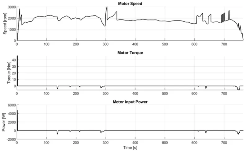
Because of the vehicle's rapid acceleration and decreased idling on interstate drives, the requirement for EM motor torque is low.

The Pack voltage, current and Soc

UDDS:

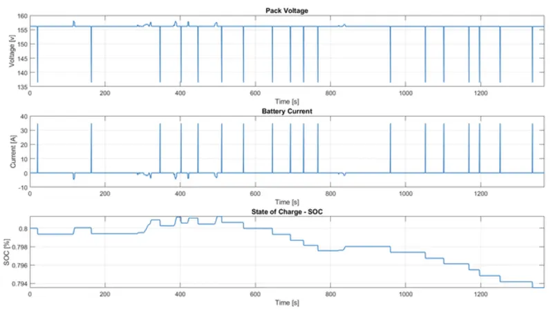
Battery SOC is responding to the motor's request for torque and the brake application by the regenerator.

The motor operating points on the motor input power map, with the motor max motoring and generating torque curves.

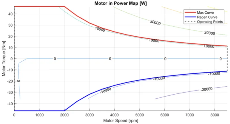
Between the maximum motoring torque curve and the maximum generating torque curve, electric motors can function.

Conclusion:

Plotting graphs and analysing the UDDS and HWFET drive cycles' various performance parameters and operating points

• Engine, transmission input, output, and wheelspeed time traces in relation to time
• Engine speed, horsepower, fuel flow, and fuel consumption increase with time.
• pedals for the accelerator and brake, desired gear and vehicle, actual speed, and vehicle distance in relation to time.
• On the engine fuel map, there are engine operating points indicated in relation to time.
• In relation to time, motor torque, speed, and input power.
• Pack voltage, current, and status of charging with regard to time.
• The motor operating points on the time-relative motor input power map as well as comparing its values with those of the HWFET driving cycle.