Week 4.1 - Genetic Algorithm

AIM:

To find global Maxima for the stalagmite function using ga(genettic algorithm) in Matlab.

ABOUT:

GA(genetic algorithm) is one of the machine learning algorithms that is used to get optimised results.

Ga is only used to create minimum solution, so the value of stalagmite function is taken as negative inorder to maximise the function.

It is a method for solving both constrained and unconstrained optimization problems based on a natural selection process that mimics biological evolution.

GA uses three types of rules at each step to create the next generation from the current population.

• selection - Selection rules select the individuals, called parents, that contribute to the population at the next generation.
• crossover - Crossover rules combine two parents to form children for the next generation.
• mutation - Mutation rules apply random changes to individual parents to form children.

Genetic Algorithm Syntax:

x = ga(fun,nvars,A,B,Aeq,Beq,lb,ub,nonlcon,options)

fun = function

nvars = no of variables

A,B = linear inequality constrains

Aeq,Beq = linear equality constrains

lb,ub = lower bound and upper bound

nonlcon = non-linear constrains

lntcon = vector of positive integers

options = optimisation options

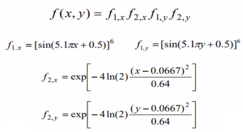
Equation for Stalagmite Function:

CODE for Stalagmite Function(Sub- Function):

Ga is only used to create minimum solution, so the value of stalagmite function is taken as negative inorder to maximise the function.

function [f] = stalagmite(input_vector)

x = input_vector(1);
y = input_vector(2);

f1 = (sin(5.1*pi*x + 0.5))^6;
f2 = (sin(5.1*pi*y + 0.5))^6;
f3 = exp(-4*log(2)*(x-0.0667)^2/0.64);
f4 = exp(-4*log(2)*(y-0.0667)^2/0.64);

f = -(f1*f2*f3*f4);

end

CODE For Finding Global Maxima:

x and y arrays are created with no of iterations

meshgrid command is used

stalagmate function is used.(-ve value is used to calculate global maxima.

tic- toc command is used to calculate the time taken.

program is splitted into 3 study's.

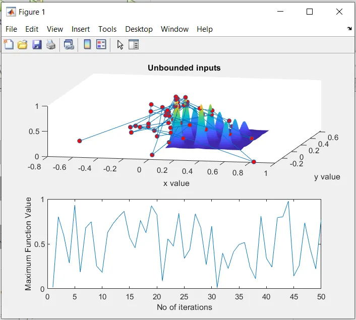
study1 - calculating global maxima by taking random samples from the function.

syntax - [inputs,fopt(i)] = ga(@stalagmite,2);

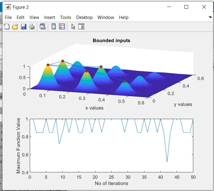
study2 - calculating global maxima by the giving boundary limits for the inputs.

syntax - [inputs,fopt(i)] = ga(@stalagmite,2,[],[],[],[],[0;0],[1;1]);

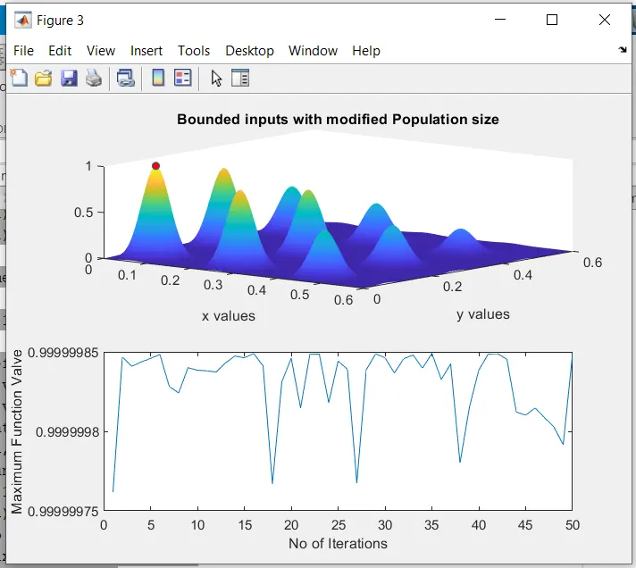
study3 - calculating global maxima by giving population size.

syntax - [inputs,fopt(i)] = ga(@stalagmite,2,[],[],[],[],[0;0],[1;1],[],[],options);

population size is set as 200.

study time is obtained.

global maxima is displayed in the workspace.

clear all
close all
clc

%defining the search space
x = linspace(0,0.6,150);
y = linspace(0,0.6,150);
num_cases = 50

%creating 2d mesh
[xx yy] = meshgrid(x,y);

%evaluating stalagmite function
for i =1:length(xx)
    for j =1:length(yy)
        input_vector(1) = xx(i,j);
        input_vector(2) = yy(i,j);
        f(i,j) = stalagmite(input_vector);
    end
end


%study1 - satistical behaviour
tic
for i = 1:num_cases
    [inputs,fopt(i)] = ga(@stalagmite,2);
    xopt(i) = inputs(1);
    yopt(i) = inputs(2);
end
study1_time = toc
subplot(2,1,1)
figure(1)
hold on
surf(x,y,-f)
xlabel('x value')
ylabel('y value')
shading interp
plot3(xopt,yopt,-fopt,'marker','o','markersize',5,'markerfacecolor','r')
title('Unbounded inputs')
subplot(2,1,2)
plot(-fopt)
xlabel('No of iterations')
ylabel('Maximum Function Value')

%study2 - Statistical behaviour with lower and upper limits
tic
for i = 1:num_cases
    [inputs,fopt(i)] = ga(@stalagmite,2,[],[],[],[],[0;0],[1;1]);
    xopt(i) = inputs(1);
    yopt(i) = inputs(2);
end
study2_time = toc
figure(2)
subplot(2,1,1)
hold on
surf(x,y,-f)
xlabel('x values');
ylabel('y values');
shading interp
plot3(xopt,yopt,-fopt,'marker','o','markersize',5,'markerfacecolor','r')
title('Bounded inputs')
subplot(2,1,2)
plot(-fopt)
xlabel('No of Iterations')
ylabel('Maximum Function Valve')

%study3 - Increasing GA iteration
options = optimoptions('ga','Populationsize',200);
tic
for i = 1:num_cases
    [inputs,fopt(i)] = ga(@stalagmite,2,[],[],[],[],[0;0],[1;1],[],[],options);
    xopt(i) = inputs(1);
    yopt(i) = inputs(2);
end
study3_time = toc
figure(3)
subplot(2,1,1)
hold on
surf(x,y,-f)
xlabel('x values');
ylabel('y values');
shading interp
plot3(xopt,yopt,-fopt,'marker','o','markersize',5,'markerfacecolor','r')
title('Bounded inputs with modified Population size')
subplot(2,1,2)
plot(-fopt)
xlabel('No of Iterations')
ylabel('Maximum Function Valve')
disp('global_maxima= ')
disp(inputs)

RESULTS:

STUDY 1

STUDY 2

STUDY 3

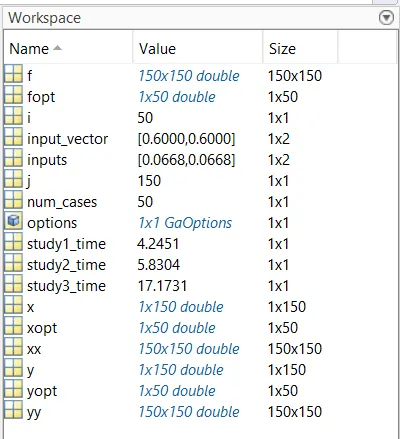
WORKSPACE:

COMMAND WINDOW:

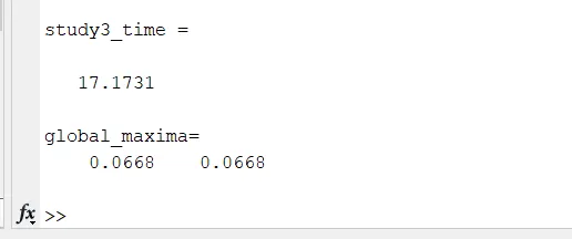
The global maxima is found out to be 0.0668