Project 2

Project2_InitFile.m” is a Matlab script used to load all the variables required for running the Simulink model and for post-processing. The drive cycle selection is also done here. Before running the Simulink vehicle model, run this initialization script.

AIM

Hybrid Vehicle Forward Model This is a simulink model which we use to simulate the vehicle. force/torque/power is the input and the vehicle state variable velocity and acceleration are outputs used for testing This is a computation testing It is mainly used to simulate a vehicle on a driving cycle to analyse the dynamic behaviour of the system helps significantly in control development. with the help It is used to moderate the performance of the vehicle during the operating time of the vehicle.

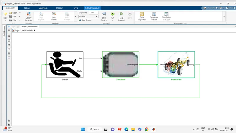
Drive Model-

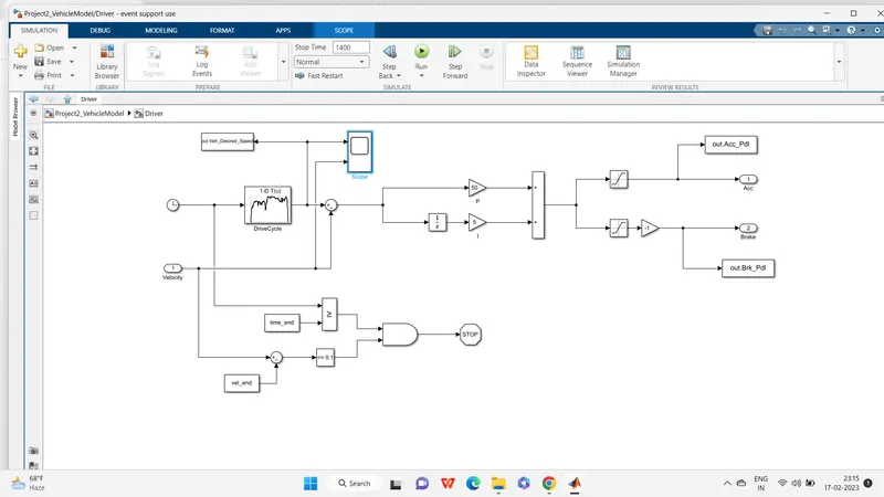
This is the input given by the driver which is in the form of controller brake and acceleration This Block is created with help of drive cycle lookup table & PID controller for correcting error signal of the feedback velocity signal, generated the Acc_pdl & Brk_pdl as output through the saturation block.

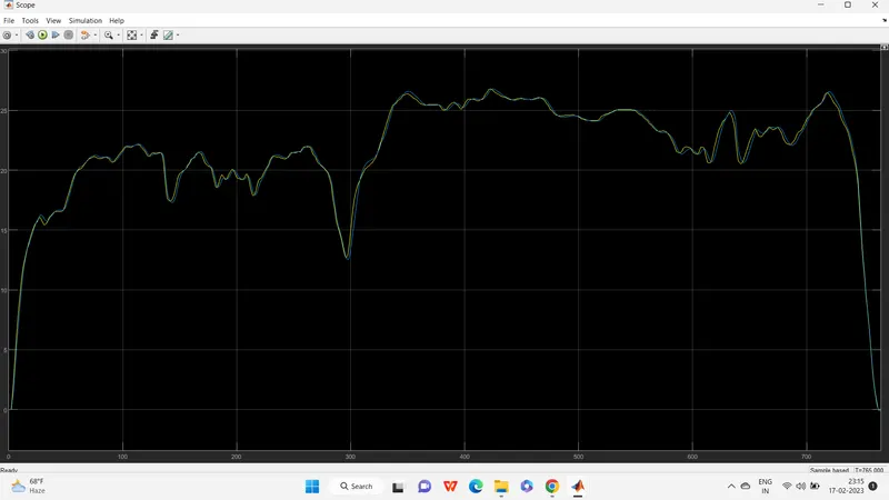
Vehicle Desired Speed and Drive Cycle in given Drive Model each other is overlapping

Controller-

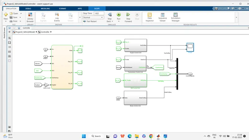
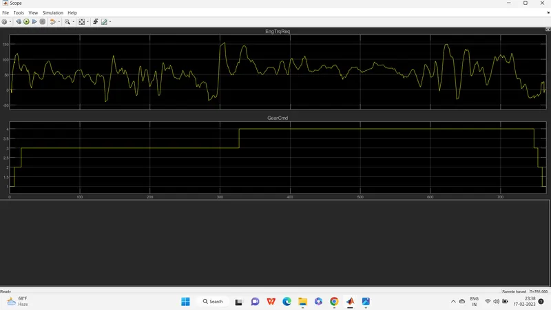
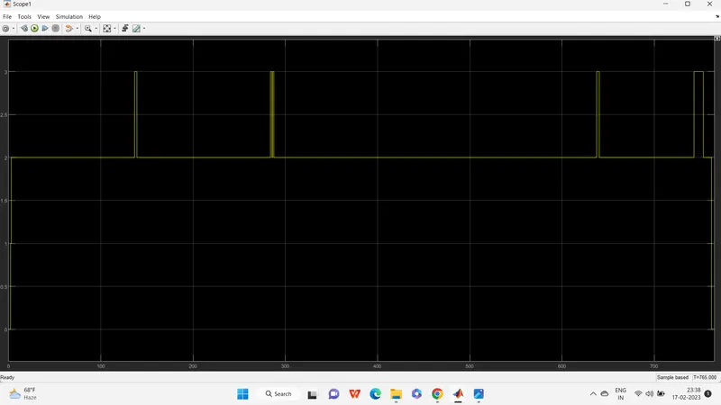
It controls the engine according to the output given by the driver turqe controls the speed of the engine Controller block having sub blocks Engine ,Transmission & Brake, vehicle velocity ,acceleration & brake signals given as inputs to the these blocks, controller block generate the output as Engine Torque, Gear command & required brake torque.

Engine Control-

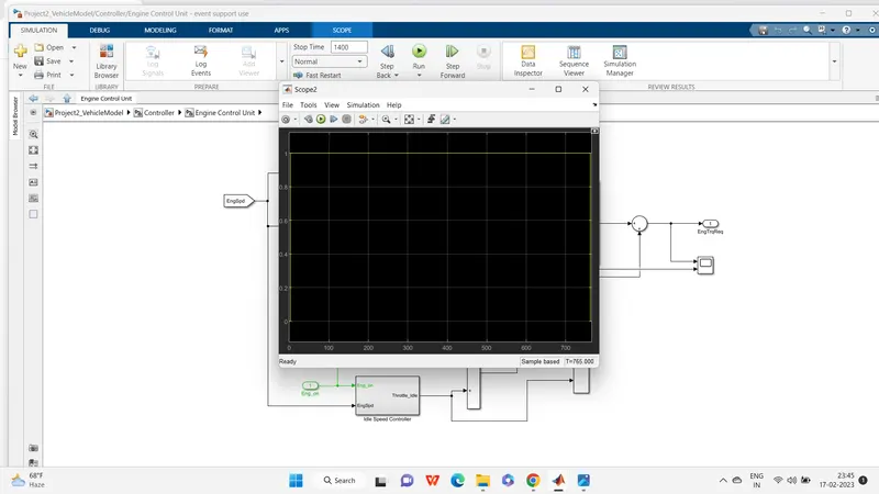
Engine control block takes the engine speed as input & gives the engine required torque as output with help of lookup blocks

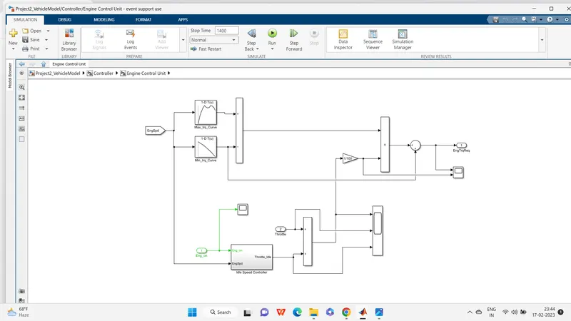
The torch and speed demanded by the vehicle driver is not always constant

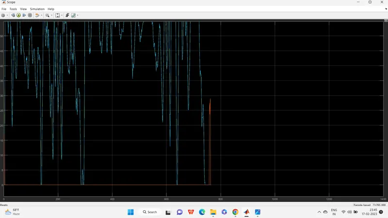
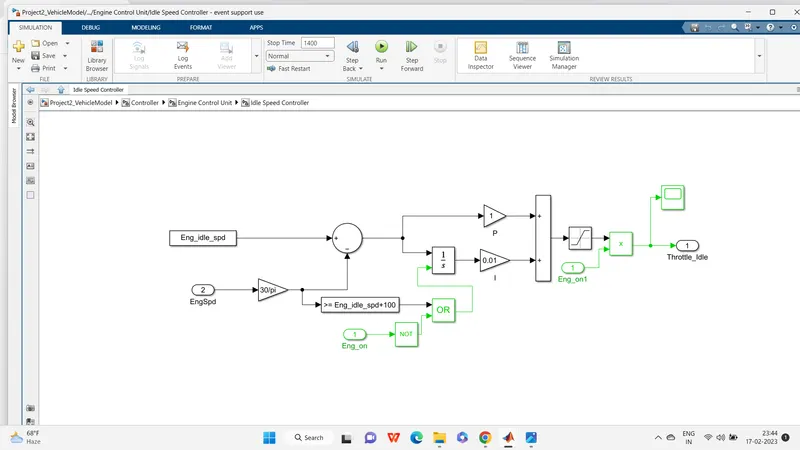
Idle Engine Speed controller-

Transmission Control-

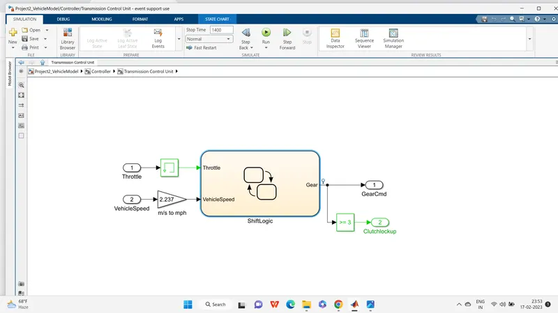
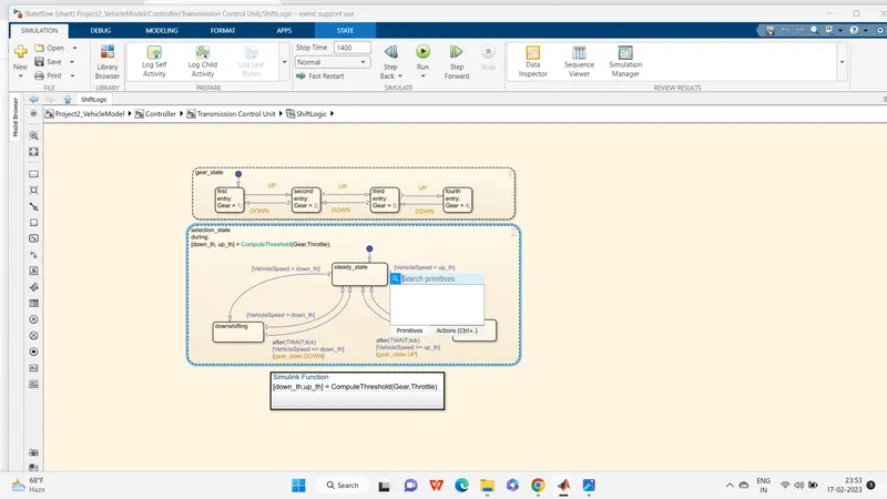
Transmission control block is created using shift logic block ,vehicle speed & Throttle given as input & Gear command taken as output of the of the transmission control block, shift logic designed based on the vehicle speed

Stateflow^® is a graphical programming environment based on finite state machines. With Stateflow, you can test and debug your design, consider different simulation scenarios, and generate code from your state machine.

Finite state machines are representations of dynamic systems that transition from one mode of operation (state) to another. State machines:

. EM Control-

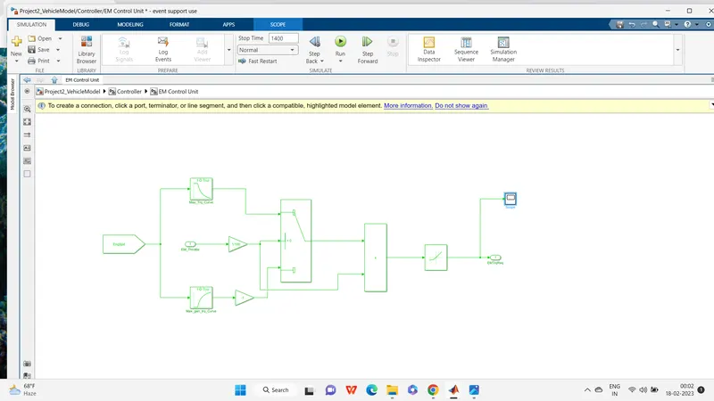
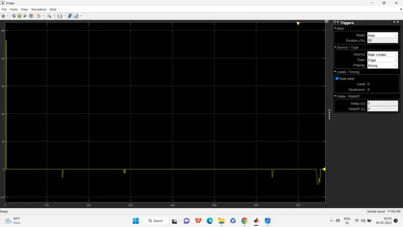
EM control block takes the engine speed as input & gives the engine required EM torque as output with help of lookup blocks

Brake Control

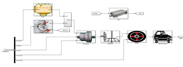
Power Train-

The component which helps in delivering the power produced by the engine to the vehicle, all the components are connected to a party cooler train, which we call the powertrain, it transmits the power produced by the engine to the wheel of the vehicle so that May we face the same tomorrow. This includes the engine, transmission, the driveshaft, differentials, axles; basically anything from the engine through to the rotating wheel

Engine-

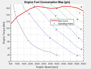
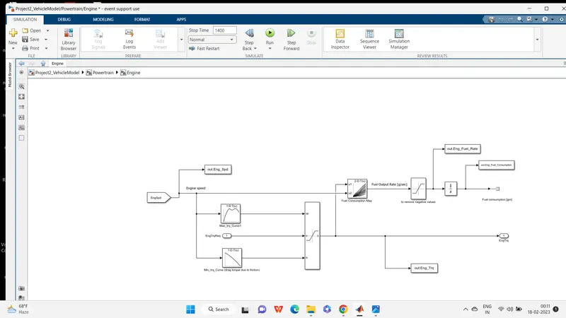
we used map based model to model the fuel consumption of engine It is based on maximum Torque and minimum torque from the controller. and then it saturated torque and give output then saturated torque and speed map give fuel consumption takes the speed and torque then the output goes into saturated then its integrated

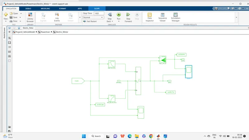
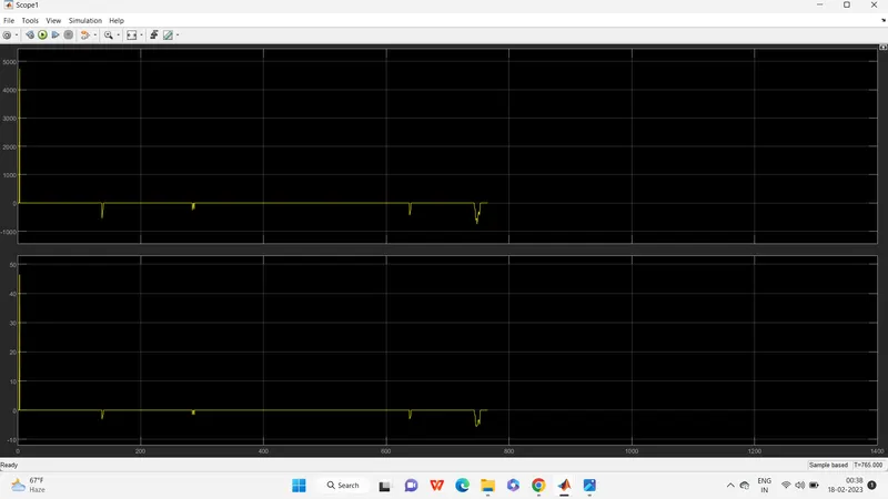
In this model we used map based model to model the Power generated by motor It is based on maximum EM Torque and generated EM torqu

Transmission—

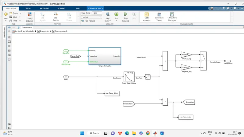
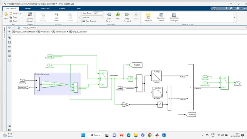
In these model we take engine torque, gear selector from controller signal for transmission of gear ratio. The ratio is multiply by transmission input torque and then the transmission efficiency positive torque and negative torque gives transmission input speed. In this case torque converter connects the engine to transmission it is part of transmission.

Torque converter-

. Differential

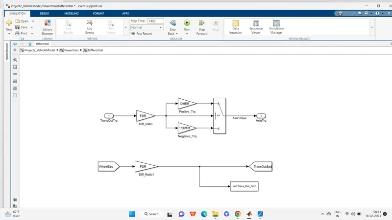
In this taking input is the transmission output then its going to the differential ratio multiplied the output and input torque then meet axle torque. The axle torque is a lower than the transmission torque and differential ratio.

Wheels

In this model we take the axle torque from differentail & brake torque from controller. it is substracted and multiplied rolling radius and velocity then we meet the tractive force from axle and brake torque. Wheel block give the wheel speed signal as output.

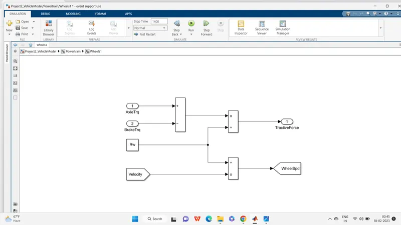
Energy Storage system

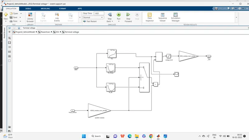
It stores the power produced by the engine and keeps it for a long time.ESS block having two sub blocks with Terminal voltage & ESS estimation blocks pack current .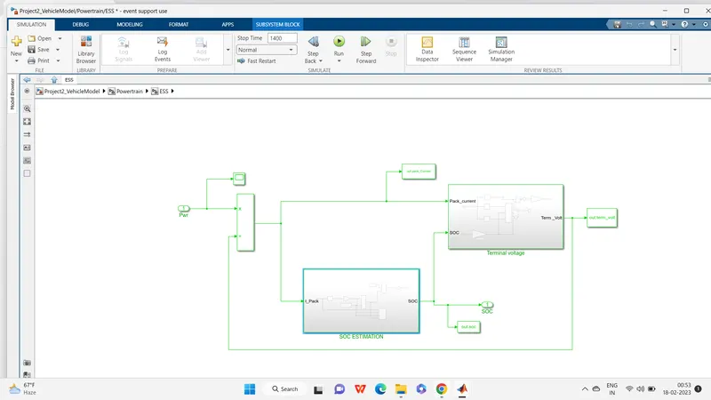

pack current is in Ampere this is integrated to get coulumbs per hour and is devided by the ESS_max_ah_cap resulted signal substared with ESS initial state of charge then its fed to stauration bolck to limit the upper & lower limits in b/w 0 to 1 .this out put SOC given as input to the voltage saturation block. with help of given data of resistance of cell during charge & discharge is given to the 1D lookup table and multiplied with current to calculate internal voltage drop across the battery cell.

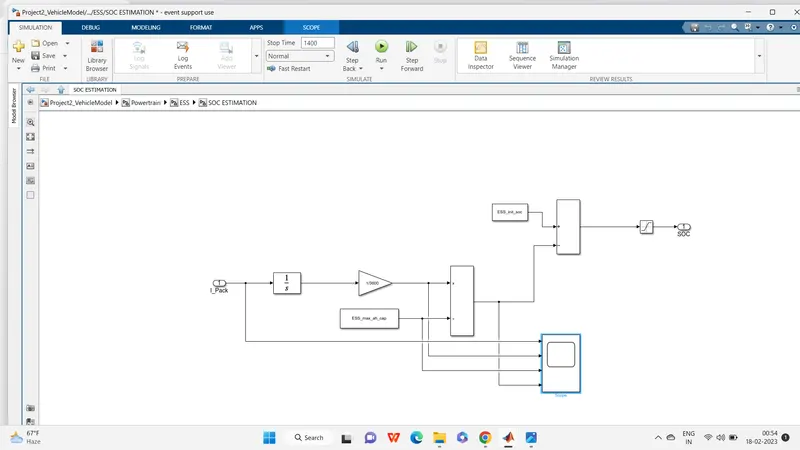
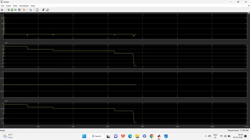
Voltage drop subtracted with open circuit voltage and multiplied with gain block to calculate the terminal voltage of 20 series battery cells.

. Vehicle Dynamics—

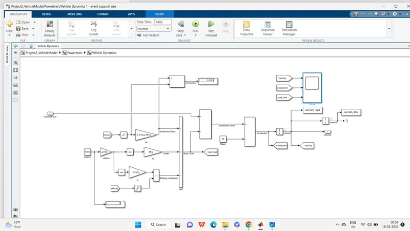
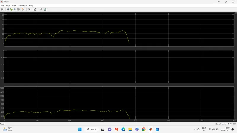
Vehicle Dynamics block designed based on the below dynamic equation (tractive force and road load) this block generates the vehicle velocity, vehicle distance as output from the block, this output vehicle velocity given to the drive block as a feedback signal

MATLAB scripts-

MATLAB scripts for plots:-

%% Skill-Lync -> Hybrid Drives Development

% Project 1 - Conventional Vehicle Model

% By - Guruprasad Joshi

%% Post-Processing File

% File for post-processing the Conventional vehicle simulation model data

%% Renaming variables

Time=out.tout;

Acc_Pdl=out.Acc_Pdl; % Accelerator pedal [%]

Brk_Pdl=out.Brk_Pdl; % Brake pedal [%]

Gear_Cmd=out.Gear_Cmd; % Transmission gear

Trans_In_Spd=out.Trans_In_Spd*30/pi; % Transmission input speed [rpm]

Trans_Out_Spd=out.Trans_Out_Spd*30/pi;% Transmission output speed [rpm]

Eng_Trq=out.Eng_Trq; % Engine brake torque [Nm]

Eng_Spd=out.Eng_Spd*30/pi; % Engine speed [rpm]

Eng_Fuel_Consump=out.Eng_Fuel_Consumption; % Engine fuel consumption [g]

Veh_Dist=out.Veh_Dist/1000; % Distance traveled by vehicle [km]

Veh_Spd=out.Veh_Spd*18/5; % Vehicle speed [kmph]

Wheel_Speed=out.Wh_Speed; % Wheel speed [kmph]

Eng_Fuel_Rate=out.Eng_Fuel_Rate % Engine fuel rate [%]

ElecPwr=out.ElecPwr;

%% Data Analysis

Eng_Pwr=Eng_Spd*(pi/30).*(Eng_Trq/1000); % Engine brake power [kW]

rho_petrol=0.7197; % Density of petrol [kg/L]

%kmpl=Veh_Dist/(Eng_Fuel_Consump/1000/rho_petrol); % Fuel economy [kmpl]

%% Plotting vehicle characteristics time trace

figure(1)

subplot(411)

hold on

grid on

plot(Time,Acc_Pdl);

ylabel('Pedal [%]');

xlabel('Time [s]');

legend('Accel');

subplot(412)

plot(Time,Brk_Pdl);

ylabel('Brk Pedal [%]')

xlabel('Time [s]');

legend('Brake');

subplot(413)

hold on

grid on

plot(Time,Gear_Cmd);

xlabel('Time [s]');

ylabel('Gear');

legend('Gear');

subplot(414)

hold on

grid on

plot(Time,Veh_Dist);

xlabel('Time [s]');

ylabel('Veh_Dist[KM]');

legend('Veh_Dist');

figure(2)

subplot(311)

hold on

grid on

plot(Time,Trans_In_Spd);

ylabel('Speed [rpm]')

legend('Trans Input');

subplot(312)

plot(Time,Trans_Out_Spd);

ylabel('Speed [rpm]')

legend('Trans Output');

subplot(313)

plot(Time,Wheel_Speed);

ylabel('Speed [rpm]')

xlabel('Time [s]');

legend('Wheel_Speed');

figure(3)

subplot(411)

plot(Time,Eng_Fuel_Consump);

ylabel('Engine fuel[g]')

legend('Eng_Fuel_Consump')

subplot(412)

plot(Time,Eng_Fuel_Rate);

ylabel('Engine fuel rate [%]')

legend('Eng_Fuel_Rate');

subplot(413)

plot(Time,Eng_Trq)

ylabel('Engine brake torque [Nm]')

legend('Eng_Trq');

subplot(414)

plot(Time,Eng_Pwr);

ylabel('Eng_Pwr [KW]')

xlabel('Time [s]');

legend('Eng_Pwr');

%% Plotting engine operating points on engine fuel map

figure('Name','Engine Operating Points');

hold on

grid on

title('Engine Operating Points','fontsize',12);

p1=plot(Eng_map_spd*30/pi,Eng_max_trq,'linewidth',2,'color','r');

p2=line([Eng_map_spd(end)*30/pi Eng_map_spd(end)*30/pi],[0 Eng_max_trq(end)]);

set(p2,'linewidth',1,'linestyle','--','color','k');

p3=line([Eng_map_spd(1)*30/pi Eng_map_spd(1)*30/pi],[0 Eng_max_trq(1)]);

set(p3,'linewidth',1,'linestyle','--','color','k');

[c,h] = contour(Eng_map_spd'*30/pi,Eng_map_trq,Eng_fuel_map');

clabel(c,h);

xlabel('Engine Speed [rpm]');

ylabel('Engine Torque [Nm]');

title('Engine Fuel Consumption Map [g/s]');

p4 = plot(Eng_Spd,Eng_Trq,'.','color','k');

legend([p1 p4],{'Max Curve','Operating Points'});

axis([Eng_map_spd(1)*30/pi Eng_map_spd(end)*30/pi 0 Eng_map_trq(end)]);

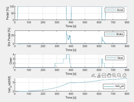
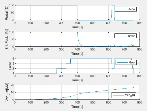
1] Plot accelerator and brake pedal, gear command, and actual speed, vehicle distance using subplots.

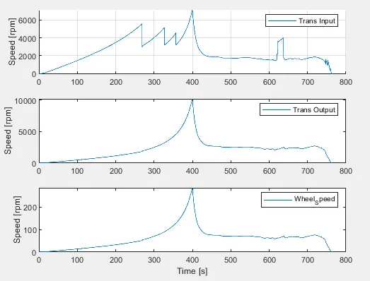
2] Plot the time trace for engine, transmission input, transmission output and wheel speed on one plot

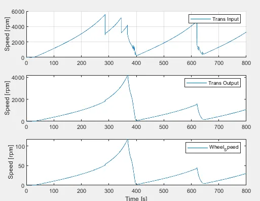
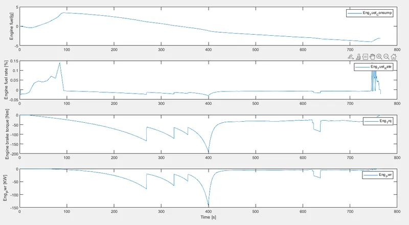
3] Plot engine torque, engine power, fuel rate and fuel consumption using subplots.

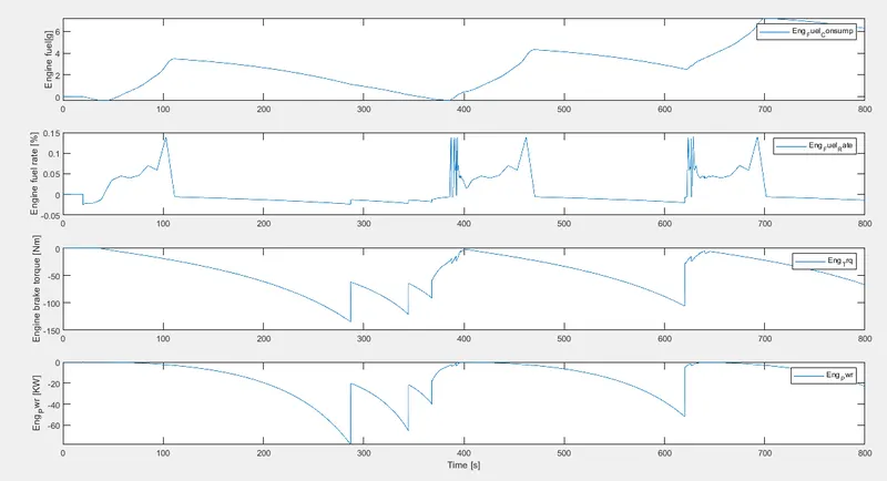
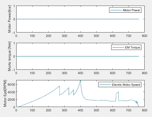
4] Plot the Motor power, Torque, Speed.

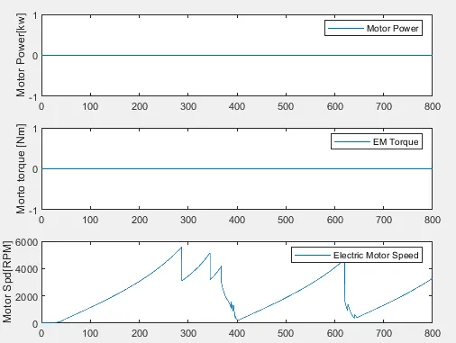
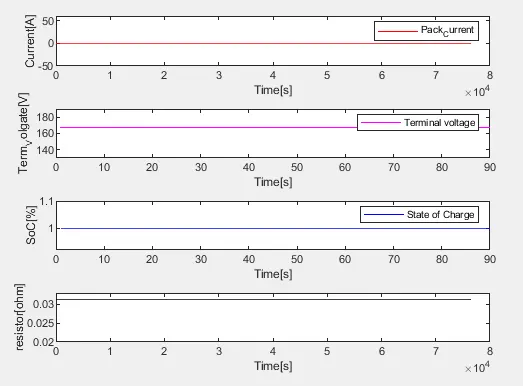
5] Plot the ESS Terminal voltage, Current, SOC, Resistor.

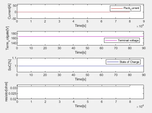
6] Plot the engine operating points on the engine fuel map.

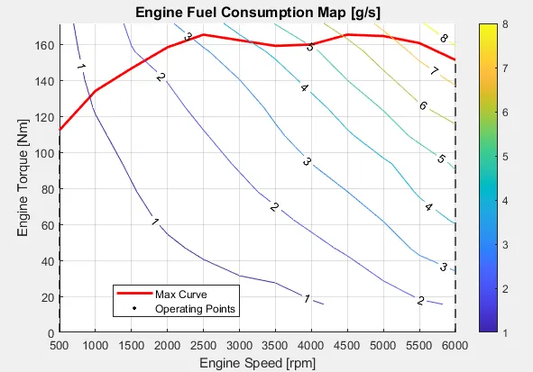
Graphs for the drive cycle HWFEET

1] Plot accelerator and brake pedal, gear command, and actual speed, vehicle distance using subplots.

2] Plot the time trace for engine, transmission input, transmission output and wheel speed on one plot

3] Plot engine torque, engine power, fuel rate and fuel consumption using subplots.

4] Plot the Motor power, Torque, Speed.

5] Plot the ESS Terminal voltage, Current, SOC, Resistor.

6] Plot the engine operating points on the engine fuel map.