Project
Aim of the project: -
To carry out a system level simulation of an All-Terrain Vehicle (AVT) using MATLAB
Objective of the project: -
It is to prepare a technical report explaining the Baja model ATV Properties with the varying conditions
Software Used
MATLAB R2020a
Body of the content: -
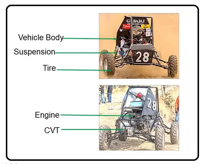
All-Terrain Vehicle (ATV): -it is also known as a quad bike or simply quad, As the name implies, it is designed to handle a wider variety of terrain than other type of vehicles these are the vehicle which travelled using low pressure tires, having a seat that is straddled by the operator along with a handlebar for steering control
E.g.: -Baja ATV
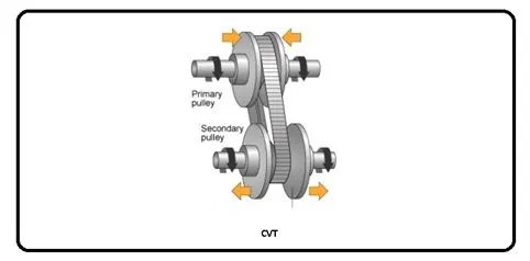
Continuously Variable transmission (CVT): - it is an automatic transmission that can change seamlessly through a continuous range of gear ratios. This contrasts with other transmissions that provide a limited number of gear ratios in fixed steps. The flexibility of a Continuous Variable Transmission with suitable control may allow the engine to operate at a constant RPM while the vehicle moves at varying speeds.
1)BAJA ALL-TERRAIN VEHICLE(ATV) without lookup table
- a) Simscape model of BAJA ATV without Dashboard
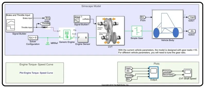
In the simscape model of BAJA ATV three main subsystems are used along with the blocks such as Engine sensors ,CVTand Vehicle body.
Blocks used in BAJA ATV
Signal builder:-it is used to provide the input signal such as Brake input ,Throttle input and to provide CVT Ratio .
Brake Input & Throttle Input
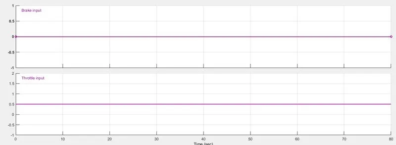
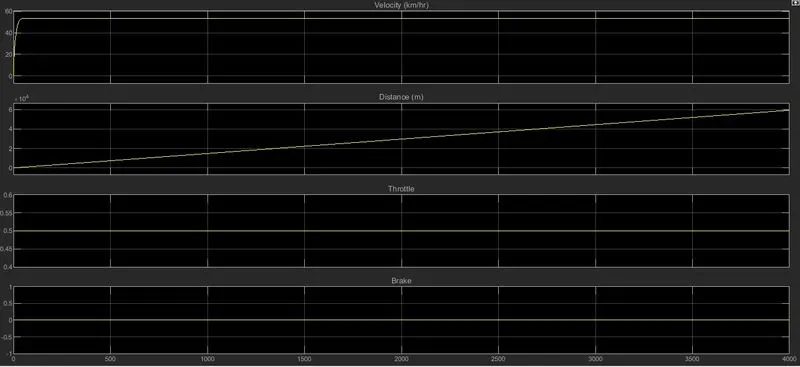
Brake input Kept Zero and the Throttle input Kept 0.5
CVT Ratio
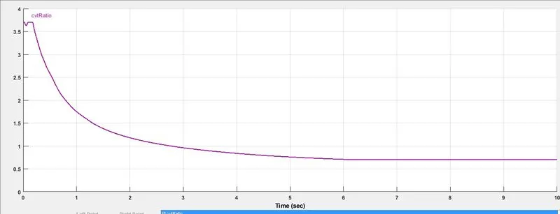
At the initial state the crt ratio kept as 3.7 and then it slitely moves down up to 3.64 then return back to 3.7it was same for fraction of seconds and starts its downword motion in the graph up to 0.7 .
Goto and From: -Goto Send signals to From block that have the specified tag.if tag visibility is ‘scoped’,then a Goto tag visibility block must be used to define the visibility of the tag.The block icon displays the selected tag name.
Solver Configuration:- Defines solver settings to use for simulation.
Mechanical Rotational Referance : -This block represents a mechanical rotational referance point ,that is,a frame or a ground.Use it to connect mechanical rotational ports that are rigidly affixed to the frame(ground).
Generic Engine:- Represents a system-level model of spark-ignition and diesel engines suitable for use at initial stages of modeling when only the basic parameters are available.Optional idle speed and redline controllers are included.The throttle input signal T lies between zero and one and specifies the torque demanded from the engine as a fraction of maximum possible torque .if the engine speed exceeds the maximum speed,the simulation stops and issues an error message.Connections F and B are mechanical rotational conserving ports associated with the engine crankshaft and engine block,respectively.Connection Pand FC are physical signal output ports through which engine power and fuel consumption rate are reported.
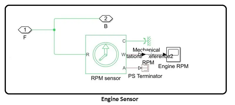
Ideal Rotational Motion Sensor: -The block kept inside the subsystem Engine sensor.it represents an ideal mechanical rotational motion sensors ,that is ,a device that converts an across variable measured between two mechanical rotational nodes into a control signal proportional to the angular velocity or angle .the sonsor is ideal since it does not account for inertia friction ,delays ,energy consumption,and so on.Connection R and C are mechanical rotational conserving ports and connections W and A are physical signal output port for velocity and angular displacement respectively.
PS Terminator: - This block is used to terminate physical signal outputs. Unconnected physical signal output port does not generate warning, but connections to PS terminator can be used to indicate that the signal was not inadvertently left unconnected.
Inertia (Input Shaft Inertia & Output shaft inertia) : - The block represents the ideal mechanical rotational inertia and here its kept under the subsystem CVT. It has one mechanical rotational conserving port. The block positive direction is from its port to the reference point. This means that the inertia torque is positive if inertia is accelerated in the positive direction.
Simple Gear: - Represents a fixed-ratio gear or gear box. No inertia or compliance is modeled in this block. You can optionally include gear meshing and viscous bearing losses.
Import: -Provide an input port for a subsystem or model. For triggered subsystems, ‘Latch input by delaying outside signal ‘produces the value of the subsystem input at the previous time step. For function call subsystems, Timing ‘On’ the Latch input for feedback signals of function-call subsystem outputs prevents the input value to this subsystem from changing during its execution. The other parameter can be used to explicitly specify the input signal attributes.
Variable Ratio Transmission/Variable Ratio Gear: -represents a variable ratio gearbox such as implemented by mechanical belt CVT, electric or hydraulic transmissions. The physical signal input r defines the ratio of input to output angular shaft velocities. Connections B(base) and F(Follower)are mechanical rotational conserving ports. Specify the relation between base and follower rotation directions with the Output shaft rotates parameter.
PS Simulink converter: - Converts the input Physical Signal to a Simulink output signal.
Simulink to PS converter: - Converts the Simulink input signal to a Physical Signal.
PS constant: - This block creates a physical signal constant.
Integrator: - Continuous-time integration of the input signal.
Tire: - Represents the longitudinal behavior of a highway tire characterized by the tire Magic Formula. The block is built from Tire-Road Interaction (Magic Formula) and Simscape Foundation Library Wheel and Axle blocks. Optionally, the effects of tire inertia, stiffness, and damping can be included. Connection A is the mechanical rotational conserving port for the wheel axle. Connection H is the mechanical translational conserving port for the wheel hub through which the thrust developed by the tire is applied to the vehicle. Connection N is a physical signal input port that applies the normal force acting on the tire. The force is considered positive if it acts downwards. Connection S is a physical signal output port that reports the tire slip. Optionally expose physical signal port M by setting Parameterize by to Physical signal Magic Formula coefficients. Physical signal port M accepts a four element vector corresponding to the B, C, D, and E Magic Formula coefficients. The parameter values Rated vertical load=2060N, peak longitudinal force at rated load=1260N, with a slip at peak foece at rated load in percent=5, with a rolling radius of 0.2921m with a tire inertia of 1e-2kg*m^2, with an initial velocity of Zero. Constant coefficient =0.015 with a velocity threshold of0.1m/s
Gain: - Element-wise gain (y = K.*u) or matrix gain (y = K*u or y = u*K).
Scope: - this block is used to display the output curves and input curve for evaluating the reports.
Double-Shoe Brake: -Represents a brake arranged as two pivoted rigid shoes symmetrically installed inside or outside a drum and operated by one actuator. The actuator force causes the shoes to exert a friction torque on a shaft connected to the drum.
Connection S is a conserving rotational terminal associated with the drum shaft. Connection F is a physical signal port representing the force input to the actuator. Positive force creates friction torque that resists shaft rotation. Optionally include thermal effects and expose thermal conserving port H by setting Thermal port to Model. Parameter values set for the Double-Shoe Brake geometry are Drum radius=150mm,
Actuator location radius=100mm, Pin location radius=125mm, pin location angle =15deg, Shoe beginning angle=5deg, Shoe span angle=120deg.In the friction section Viscous friction coefficient=0.01Nm/(rad/s), thermal port set as Omit, Contact Friction coefficient =0.3 with an angular velocity threshold of 0.01rad/sec.
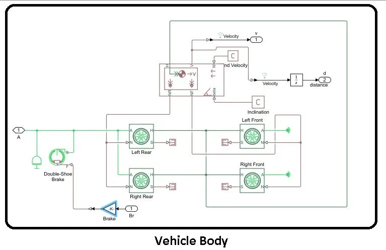
Vehicle Body: -Represents a two-axle vehicle body in longitudinal motion. The block accounts for body mass, aerodynamic drag, road incline, and weight distribution between axles due to acceleration and road profile. The vehicle can have the same or a different number of wheels on each axle. Optionally include pitch and suspension dynamics or additional variable mass and inertia. The vehicle does not move vertically relative to the ground. Connection H is the mechanical translational conserving port associated with the horizontal motion of the vehicle body. The resulting traction motion developed by tires should be connected to this port. Connections V, NF, and NR are physical signal output ports for vehicle velocity and front and rear normal wheel forces, respectively. Wheel forces are considered positive if acting downwards. Connections W and beta are physical signal input ports corresponding to headwind speed and road inclination angle, respectively. If variable mass is modeled, the physical signal input ports CG and M are exposed. CG accepts a two- element vector representing the x and y distance offsets from vehicle CG to additional load mass CG. M represents the additional mass. If both variable mass and pitch dynamics are included, the physical signal port J accepts the inertia of the additional mass about its own CG.mass set for the vehicle body is 250kg with 2 number of wheels per axle ,Horizontal distance from CG to front axle=1m, horizontal distance from CG to rear axle=0.35m, CG height above ground=0.7, Externally-defined additional mass kept as off ,gravitational acceleration =9.81m/s^2,with a frontal area of0.735482 m^2, Drag coefficient=1.92, air density = 1.18kg/m^3
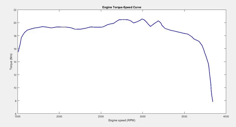
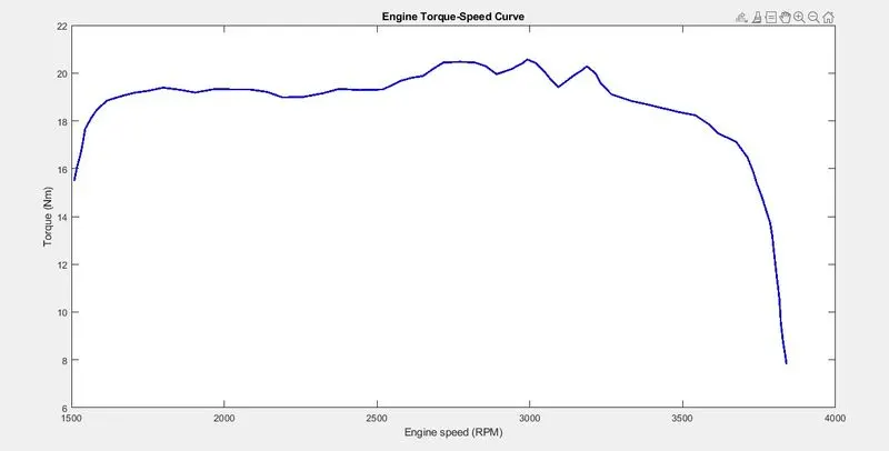
Engine Torque with respect to engine speed (RPM) curve is
After running the Simulink model with the specified inputs given through signal builder we will get an output value of velocity and distance along with the input values of throttle and brake as given below
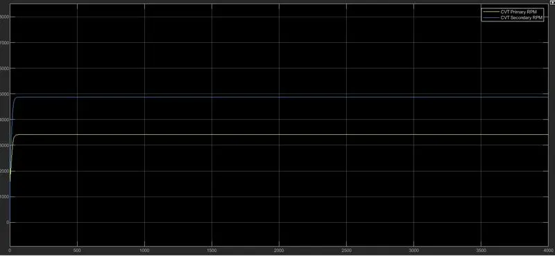
CVT shaft speed also displayed by the scope function as given below
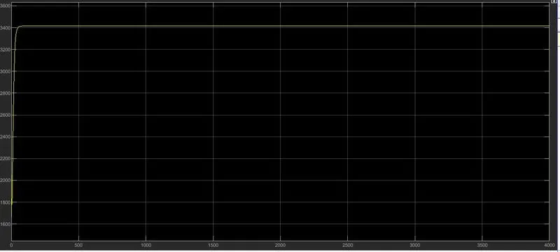
RPM (with respect to time) produced by the engine is displayed by the scope block in the Engine system subsystem as shown below.
b)Baja ATV model With Dashboard.
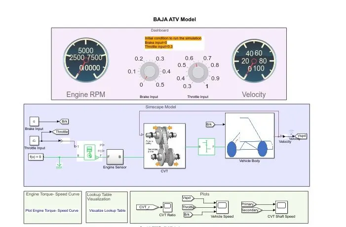
Dashboard is the control panel located in front of vehicle driver/operator, which will display the controlling and monitoring instruments The Simulink model of Baja ATV with dashboard is shown below
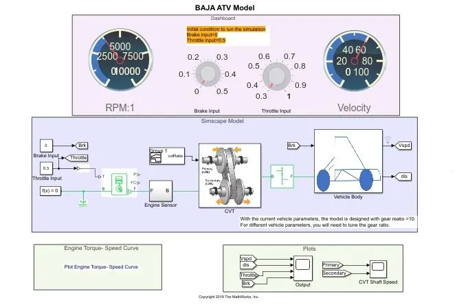
Additional Blocks available in this Simulink model are
Knob: -Set a value to tune parameters or variables for braking and also to give throttle input, at initial condition the brake set as zero and throttle set as 0.3, the maximum value is 0.5 for brake and 1 for throttle
Custom Gauge: -Display an input value on a customized gauge.
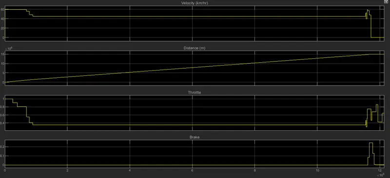
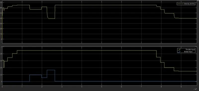
Output curve velocity, distance, throttle, brake with respect to time displayed by the scope block after the simulation with varying throttle and brake as shown below
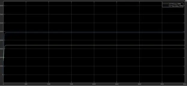
CVT shaft speed for primary and secondary shaft is as shown below with the varying condition of throttle and brake
 In our case the maximum value produced for primary and secondary shaft is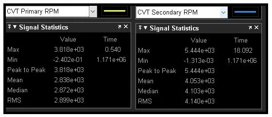
CVT Engine speed curve is shown below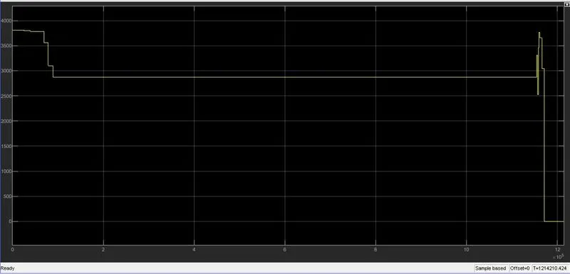
2BAJA ATV Model with lookup table
2.a) BAJA ATV without Dashboard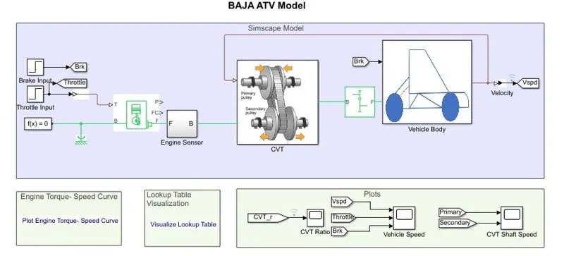
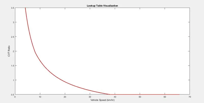
PS Lookup table: - This block represents a physical signal converter whose input-output relationship is specified a lookup table. The table grid must be in strictly scenting or strictly descending order, but the spacing can be nonuniform. Right-click on the block and select Foundation Library > Plot Table to visualize the table data based on the selected interpolation and extrapolation methods.
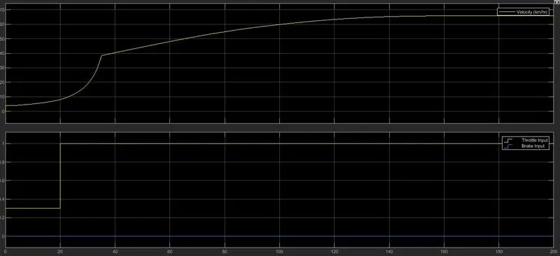
Step: - used to give stepped input values for brake step time set as 35 and all other parameters kept zero. But in the case of throttle step time kept as 20 with an initial value of 0.3 to the final value of 1
Simulink Design inside Subsystem CVT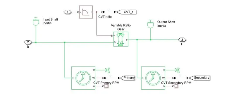
Visualization of lookup table is shown below
Engine Torque Speed Visualization curve is
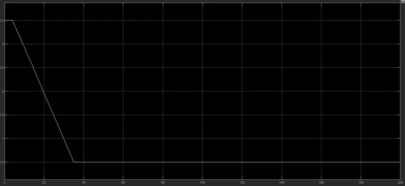
CVT ratio graph is shown below
Vehicle Velocity, brake, throttle curve with respect time is as shown below
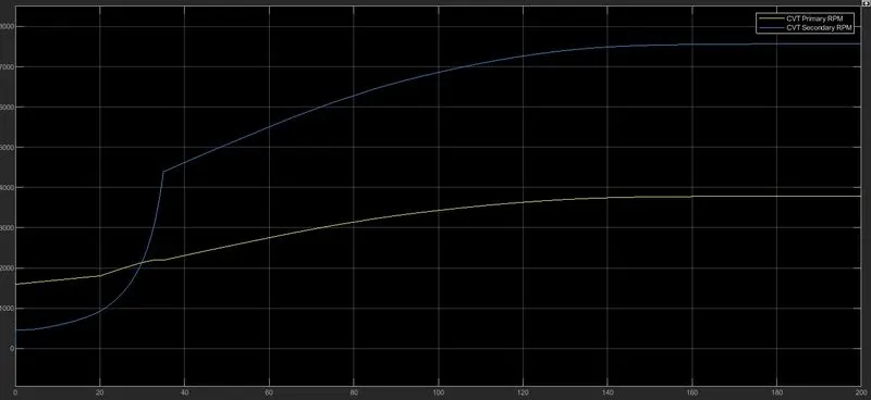
CVT Shaft speed curve of Primary CVT shaft and Secondary CVT shaft is shown below
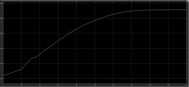
Engine RPM curve
2b) BAJA ATV with Dashboard and lookup table
Simulink model of BAJA ATV with dashboard and lookup table is shown below,like BAJA ATV with dashboard and without lookup table , the value of throttle and brake varied by two separate knobs.
CVT Ratio curve 
Velocity, throttle and braking curve with the respected time is shown below
CVT shaft speed curve 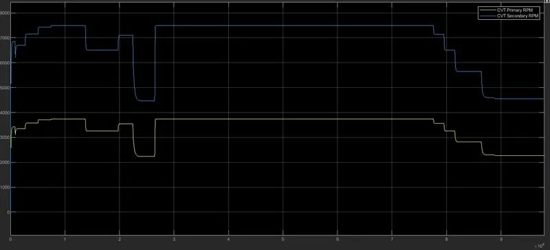
Engine speed curve with respect to time
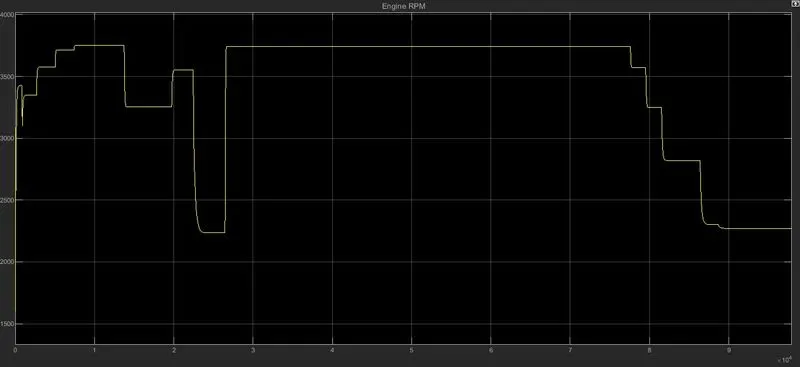
While varying the throttle value the value of the engine speed also varying.
Conclusion: - it is concluded that the vehicle speed and velocity is directly proportional to the throttle value given and its inversely proportional to the braking value applied and the speed value getting stable or stopped after reaching the maximum engine RPM