Aim- To conduct a system-level simulation of continuously variable transmission of an ATV

Objectives-

1. To understand the working of the CVT model
2. To explore the various blocks used for modelling a BAJA ATV
3. To perform simulation and compare results with or without using lookup tables

Introduction-

A continuously variable transmission (CVT) is a type of automatic transmission that can change through a continuous wide range of gear ratios. This flexibility of a CVT to provide infinite number of gear ratios allows the engine to operate at a constant RPM while the vehicle moves at varying speeds. CVT is fairly a mature technology. The world’s first CVT was Variomatic, patented and produced commercially by Hub van Doorne in the late 1950s.

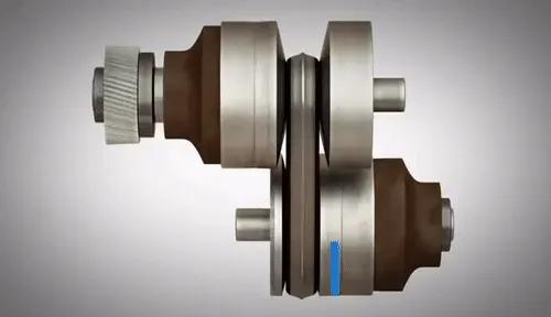
CVT does not make use of gears. Instead, it has two pulleys, whose diameters are variable and are connected by a belt. One end is connected to the engine and the other one is connected directly to the wheels or to a gearbox, where the power is delivered. The pulleys are movable and as they come closer to each other, the belt rides higher making the diameters of the pulleys larger and vice-versa.

Use of CVT in BAJA SAE® ATVs-

BAJA SAE® ATVs have to go through a variety of dynamic events including sledge pulls, acceleration tests, hill climbs and rugged suspension tracks. To be able to handle such dynamic test the powertrain must designed in such a way to handle these conditions and operate in an effective way. All BAJA SAE® teams are given a Briggs and Stratton 10 HP engine so the challenge lies in how a particular uses this power. The final event, endurance race puts challenges from all the dynamic events.

A CVT has all the advantages needed for a BAJA competition, it can efficiently adjust & reacts quickly to varying load conditions.

Model Explanation-

Here we are dealing with two types of models-

• OPEN LOOP MODEL
• CLOSED LOOP MODEL

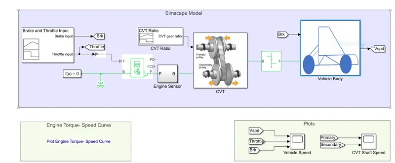
Figure 1: Open Loop model without dashboard

OPEN LOOP MODEL- (without dashboard)

This model uses the following blocks for modelling the system.

Block	Directory	Use
Signal Builder	Simulink/Sources	Create and generate interchangeable piecewise linear groups of signals
Goto	Simulink/Signal Routing	Passes its input to its corresponding From blocks.
Solver Configuration	Simscape / Utilities	Defines solver settings to use for simulation.
Mechanical Rotational Reference	Simscape / Foundation Library / Mechanical / Translational Elements	Block represents a mechanical rotational reference point.
Simulink P-S Converter	Simscape / Utilities	Converts the Simulink input signal to a Physical Signal.
Generic Engine	Simscape/Driveline/Engines	Internal combustion engine with throttle, rotational inertia and time lag
Ideal Rotational Motion Sensor	Simscape / Foundation Library / Mechanical / Mechanical Sensors	Represents an ideal mechanical rotational motion sensor.
Scope	Simulink/Sink	Output range of input values with sample time.
PS Terminator	Simscape / Foundation Library / Physical Signals / Sinks	Terminator for unconnected physical signal outputs
Inertia	Simscape / Multibody / Body Elements	Represents an ideal mechanical translational inertia
Variable Ratio Transmission	Simscape / Driveline / Couplings & Drives	Dynamic gearbox with variable and controllable gear ratio, transmission compliance, and friction losses
Simple Gear	Simscape / Driveline / Gears	Represents a fixed-ratio gear without inertia or compliance.
From	Simulink/Signal Routing	Accepts a signal from a corresponding Goto block
Inport	Simulink/Sources	Create input port for subsystem or external input
Double-shoe Brake	Simscape / Driveline / Brakes & Detents / Rotational	Frictional brake with two pivoted shoes diametrically positioned about a rotating drum with triggered faulting
Gain	Simulink/Math Operations	Multiplies the input by a constant value
MATLAB Function	Simulink/User-defined function	Allows to create function using MATLAB script.
Tire (Magic formula)	Simscape / Driveline / Tires & Vehicles	Tire with longitudinal behaviour given by Magic Formula coefficients
Rotational free end	Simscape / Foundation Library / Mechanical / Rotational Elements	Rotational port terminator with zero torque
Vehicle body	Simscape / Driveline / Tires & Vehicles	Two-axle vehicle with longitudinal dynamics and motion and adjustable mass, geometry, and drag properties
P-S Simulink Converter	Simscape / Utilities	Converts the Physical Signal to a Simulink signal.
PS Constant	Simscape / Foundation Library / Physical Signals / Sources	Generate constant physical signal
Outport	Simulink / Sinks	Create output port for subsystem or external output

In this model the throttle & brake inputs are given using signal builder to the generic engine block, it is further connected to a solver configuration. The engine rpm is then given as input to the CVT subsystem and the CVT ratios are provided using signal builder.

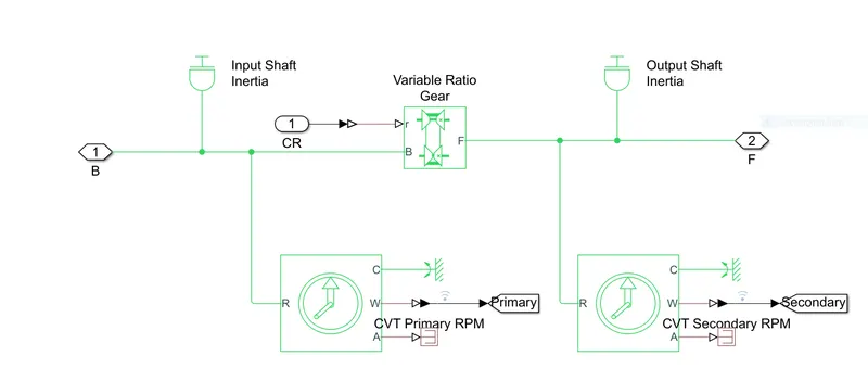
Figure 2: CVT subsystem of the model

CVT subsystem consists of inertia blocks to model the inertia of the CVT pulleys which are connected to a variable ratio transmission block

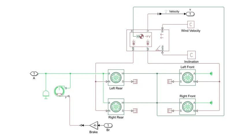
Figure 3: Vehicle body subsystem

The output from CVT is connected to a simple gear block which is further connected to the vehicle body subsystem which comprises vehicle body block, tire and brake.

The vehicle body is modelled by using the vehicle body block

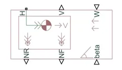
Figure 4: Vehicle Body Block

It consists of six ports for modelling different aspects of vehicle body.

H	Hub is used to connect Hubs of the wheel to the main body of the vehicle.
V	Velocity is used to output the speed/velocity at which the vehicle is moving.
W	Wind acting on the vehicle by giving a speed for it.
NR	Normal forces of rear wheel
NF	Normal forces of front wheel.
beta	Inclination angle for hill climbing force.

Tire is modelled using the magic formula

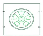
Figure 5: Tire (Magic formula)

It has 4 ports and these are –

N	Normal force acting on the tyre.
S	Slip acting on the tire.
A	Mechanical rotational port associated with the axle that the tire sits on.
H	Mechanical translational port associated with the wheel hub that transmits the thrust generated by the tire to the remainder of the vehicle.

Inputs like throttle, brake and CVT ratio were given with the help of signal builder block. The brake signal is set at zero such that no braking takes place, the throttle is given as 0.3 for 20 sec and then increases to 1 for rest of the simulation. The CVT gear ratio as maintained as 3.1 for 4 sec and then linearly decreases to 0.5 and stays constant throughout.

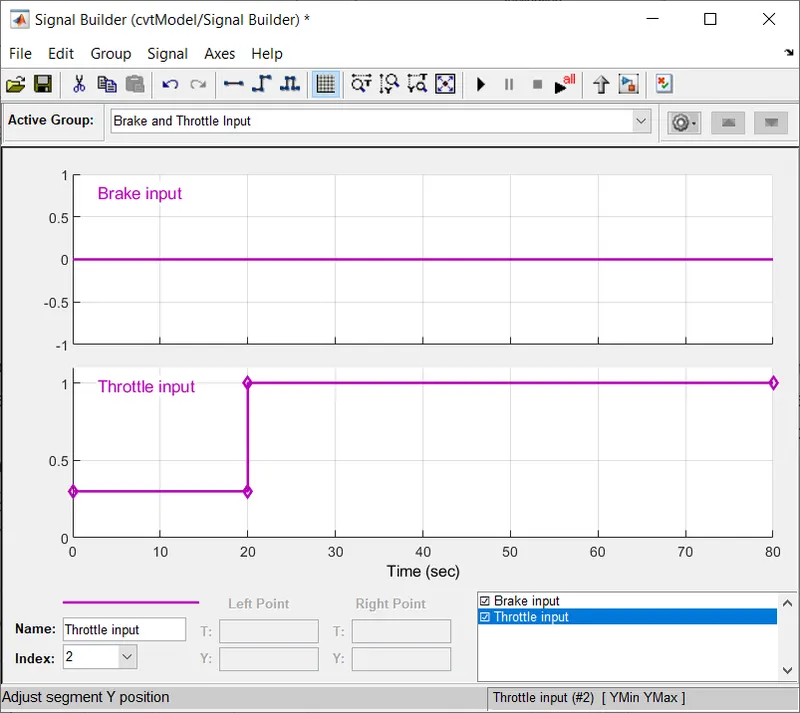
Figure 6: Brake and throttle input

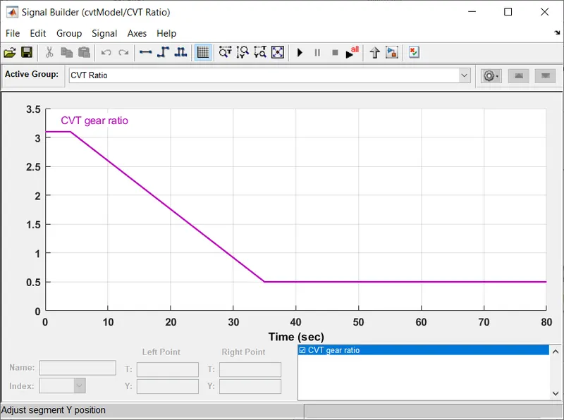
Figure 7: CVT gear ratio

The engine is modelled by using the speed-torque characteristics of BAJA engine.

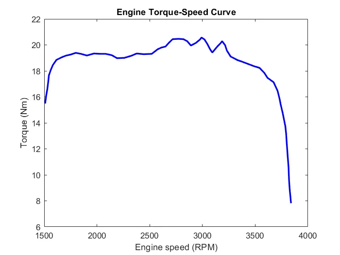
Figure 8: BAJA engine characteristics

0PEN LOOP MODEL- (with dashboard)

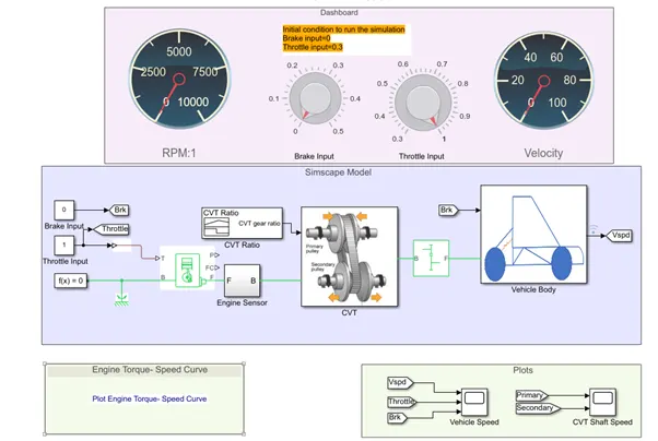
Figure 9: Open loop model with dashboard

This is exactly similar to the one discussed above without dashboard, the difference here being is that brake and throttle inputs can be given in real time while the simulation is running with the help of knobs.

CLOSED LOOP MODEL- (without dashboard)

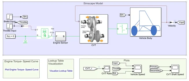
Figure 10: Closed loop model without dashboard

This is a closed loop model, where the output vehicle speed is given as input to the primary pulley of the CVT. The model extracts the CVT ratio from vehicle speed by making use of look-up table.

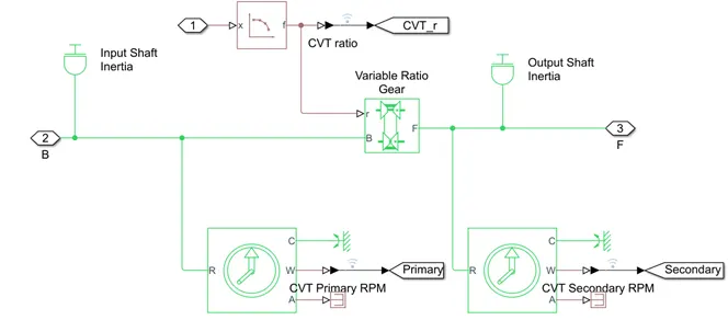
Figure 11: CVT subsystem with lookup table

CLOSED LOOP MODEL- (with dashboard)

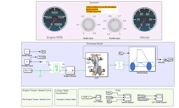
Figure 12: Closed loop model with dashboard

Lookup Table-

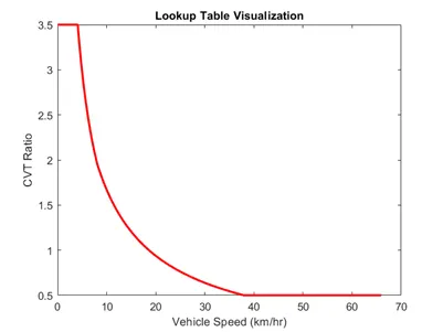
Figure 13: Lookup table showing relation between CVT ratio and Vehicle speed

Results-

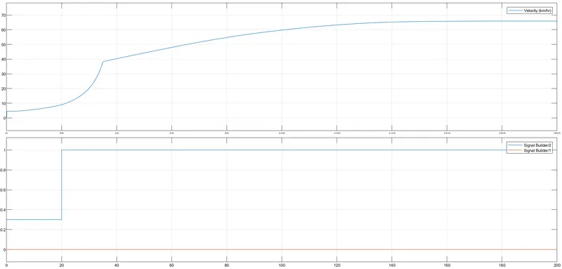
Figure 15: Vehicle Speed and throttle/brake inputs

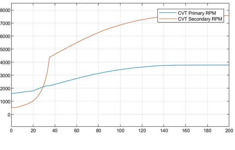
Figure 14: CVT RPM

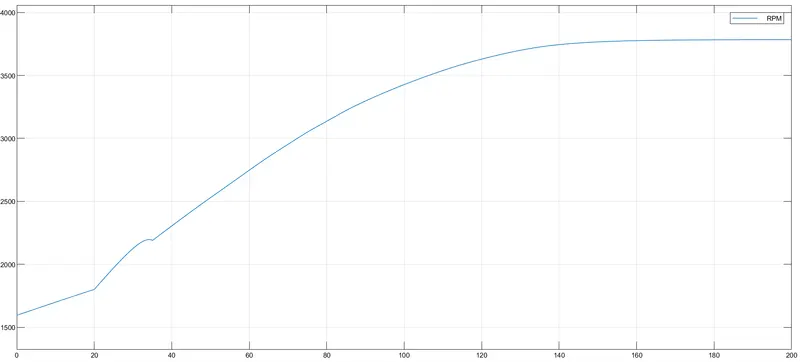
Figure 16: Engine RPM

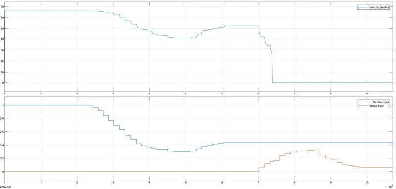
Figure 17: Vehicle Speed and throttle/brake inputs using dashboard

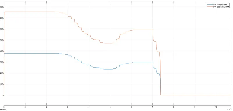
Figure 18: CVT RPM using dashboard

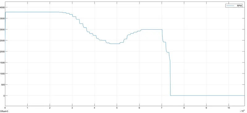
Figure 19: Engine RPM using dashboard

Observations-

1. As the throttle value is increased the velocity of the vehicle is increased which in turn increases the engine rpm thereby increasing the power.
2. As the brake input is increased the velocity is decreased and the engine rpm is also decreased.
3. As the CVT ratio increases the vehicle speed decreases.

Conclusion-

The system level simulation of BAJA ATV with CVT has been performed successfully. This project gave a deep analysis of powertrain design parameters, their dependencies onto one another. The key takeaways from this project include use of MATLAB/SIMULINK for carrying out simulations to get the intended output as per design and calculations beforehand. The fidelity of the model can be improved by using real component data and also by using better vehicle dynamic models.