Project on system-level simulation of an All-Terrain Vehicle (ATV) using MATLAB/Simulink
A system-level simulation of an all-terrain vehicle (ATV) in Simulink
AIM: To carry out a system-level simulation of an all-terrain vehicle used in BAJA
OBJECTIVE:
To prepare a full detail technical report on the BAJA (ATV) model with the Continous Variable Transmission (CVT).
(1) Simulink model of ATV without a lookup table.
(2) Simulink model of ATV with a lookup table.
BRIEF:
All-Terrain Vehicle:
An all-terrain vehicle (ATV), also known as a light utility vehicle (LUV) a quad bike, or simply a quad, as defined by the American National Standards Institute (ANSI); is a vehicle that travels on low-pressure tires, with a seat that is straddled by the operator, along with handlebars for steering control. As the name implies, it is designed to handle a wider variety of terrain than most other vehicles. Although it is a street-legal vehicle in some countries, it is not street-legal within most states, territories, and provinces of Australia, the United States or Canada.
By the current ANSI definition, ATVs are intended for use by a single operator, although some companies have developed ATVs intended for use by the operator and one passenger. These ATVs are referred to as tandem ATVs.
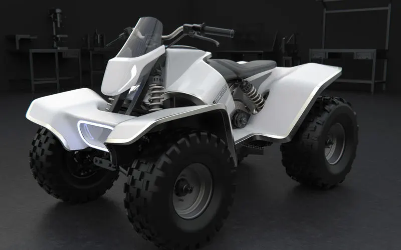
fig(i). A basic model of AVT
The rider sits on and operates these vehicles like a motorcycle, but the extra wheels give more stability at slower speeds. Although most are equipped with three or four wheels, six-wheel models exist for specialized applications. Multiple-user analogues with side-by-side seating are called utility terrain vehicles (UTVs) or side-by-sides to distinguish the classes of vehicle. Both classes tend to have similar powertrain parts. Engine sizes of ATVs currently for sale in the United States (as of 2008 products) range from 49 to 1,000 cc (3.0 to 61 cu in).
Continuously Variable Transmission (CVT):
A continuously variable transmission (CVT) is an automatic transmission that can change seamlessly through a continuous range of gear ratios. This contrasts with other transmissions that provide a limited number of gear ratios in fixed steps. The flexibility of a CVT with suitable control may allow the engine to operate at a constant RPM while the vehicle moves at varying speeds.
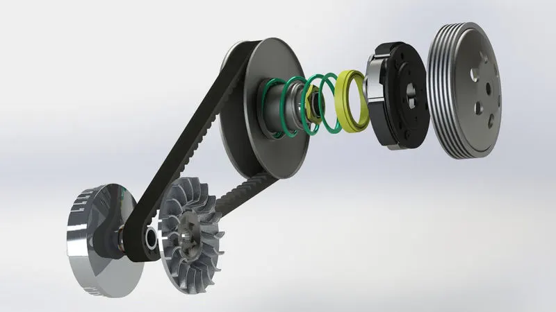
fig(ii). The exploded view of the CVT system
CVTs are used in automobiles, tractors, motor scooters, snowmobiles, and earthmoving equipment.
The most common type of CVT uses two pulleys connected by a belt or chain, however, several other designs have also been used at times. The basic CVT running is shown below. The blue is the primary CVT and the red is the secondary CVT.
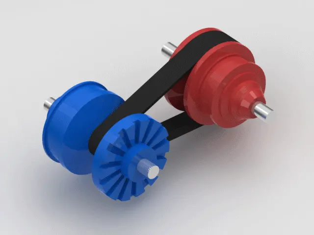
fig(iii). Working of a CVT system
SAE BAJA:
Baja SAE is a Collegiate Design Series competition run by the Society of Automotive Engineers International (SAE International). Teams of students from universities all over the world design and build small off-road cars. The cars all have engines of the same specifications. As of 2018, the engine has been an unmodified Briggs & Stratton Model 19 Vanguard engine single-cylinder with a displacement of 305cc and power output of approximately 10 bhp (7.5 kW).
The goal in Baja SAE racing is to design, build and race off-road vehicles that can withstand the harshest elements of rough terrain. The vehicles used in Baja SAE racing are often similar in appearance to dune buggies.
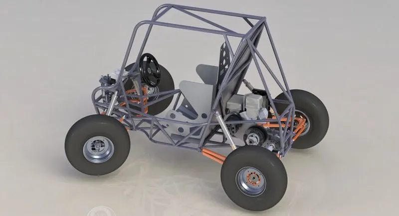
fig(iv). CAD design of a BAJA SAE model
EXPLANATION:
PART 1: Simulink model of ATV without a lookup table:
(1) ATV Model without a dashboard:-
The below figure represents the Simulink model for the BAJA ATV using the CTV for power transmission.
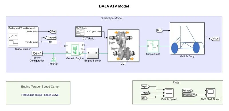
fig(v). Simulink Layout of AVT model
Blocks used:-
(I) Signal Builder: It is used to display, create, and edit interchangeable groups of signal sources and quickly switch the groups into and out of a model. We can define any piecewise linear signal shape (waveform) to assign the required input. In this model, we have used two signal builder blocks, one for brake & throttle input and another for CVT Ratio.
a. Brake & Throttle Input:
fig(vi) Signal builder for brake and throttle input
b. CVT Ratio:
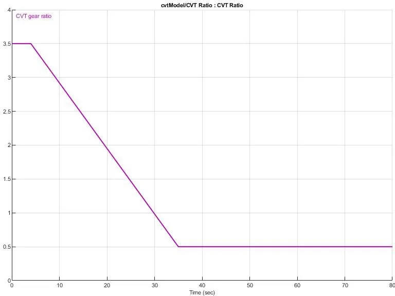
fig(vii). Signal builder for CVT gear ratio
(II) Generic Engine:
The Generic Engine block represents a general internal combustion engine. Engine types include spark-ignition and diesel. Speed-power and speed-torque parameterizations are provided. A throttle physical signal input specifies the normalized engine torque. Optional dynamic parameters include crankshaft inertia and response time lag. A physical signal port outputs engine fuel consumption rate based on the choice of fuel consumption model. Optional speed and redline controllers prevent the engine to stall and enable cruise control.
| Port Name | Description | |||||||
| B | Rotational conserving port representing the engine block | |||||||
| F | Rotational Conserving port representing the engine crankshaft | |||||||
| T | Physical signal input port specifying the normalized engine throttle level | |||||||
| P | Physical signal output port reporting the instantaneous engine power, in W | |||||||
| FC | Physical signal output port reporting the fuel consumption rate, in kg/s | |||||||
The throttle input signal T lies between zero and one and specifies the torque demanded from the engine as a fraction of the maximum possible torque. If the engine speed falls below the Stall speed, the engine torque is blended to zero. If the engine speed exceeds the maximum speed, the simulation stops and issues an error message.
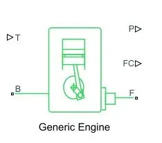
Connections F and B are mechanical rotational conserving ports associated with the engine crankshaft and engine block, respectively. Connections P and FC are physical signal output ports through which engine power and fuel consumption rate are reported.
(III) CVT:
The CVT block is the representation of the actual continuous variable transmission system having subsystems into it.
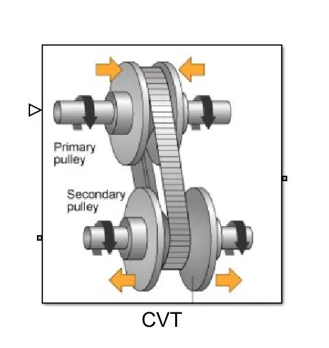
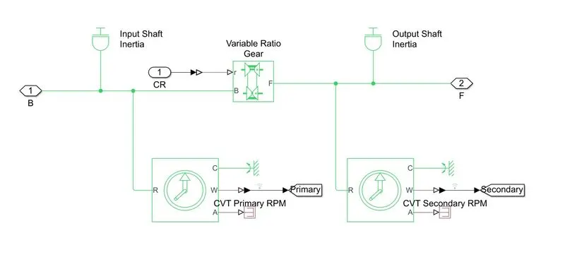
fig(viii) Subsystem of CVT
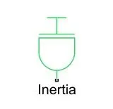
a. Interia block: It represents an ideal mechanical rotational inertia and it has one or two mechanical rotational conserving ports. The difference is purely graphical, as the ports are rigidly linked. The block positive direction is from its port to the reference point. This means that the inertia torque is positive if the inertia is accelerated in a positive direction. In this, there are two inertia blocks, one at the input and another one at the output.
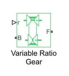
b. Variable ratio gear: It represents a variable ratio gearbox such as implemented by mechanical belt CVT, electric, or hydraulic transmissions. The physical signal input r defines the ratio of input to output angular shaft velocities. Connections B (base) and F (follower) are mechanical rotational conserving ports. Port B is connected to the PMC (Physical Modelling Connection) signal as input and Port F is output PMC port on the right side of the block with two inertia blocks at entry and exit.
c. Ideal rotational motion sensor: This block measures angular velocity or angle in a mechanical rotational network. The sensor is ideal since it does not account for inertia, friction, delays, energy consumption, and so on. The physical signal ports W and A report the angular velocity and angular displacement, respectively, of port R relative to port C. The measurement is positive when the motion at R is greater than the motion at C. The one block at the entry of variable ratio gear block and another at the exit.

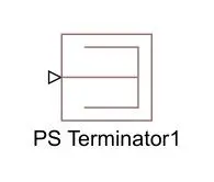
d. PS terminator and Mechanical rotational references connected to the Port A and C of the Ideal rotational block.
(IV) Vehicle Body:
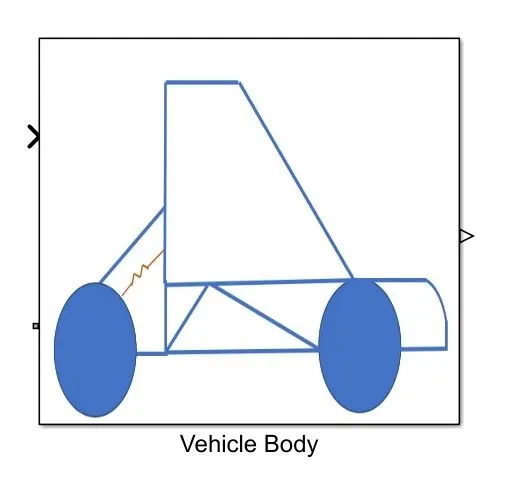
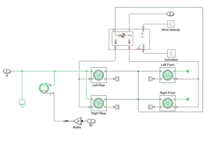
The vehicle body block represents the complete vehicle assembly with all the inputs required to operate the engine with the varying parameters. The subsystem of the vehicle is explained below:
fig(ix) Subsystem of the Vehicle body
a. Vehicle body:
This block represents a two-axle vehicle body in longitudinal motion. The block accounts for body mass, aerodynamic drag, road incline, and weight distribution between axles due to acceleration and road profile. The vehicle can have the same or a different number of wheels on each axle. Optionally include pitch and suspension dynamics or additional variable mass and inertia. The vehicle does not move vertically relative to the ground.
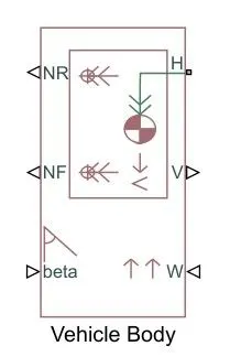
Connection H is the mechanical translational conserving port associated with the horizontal motion of the vehicle body. The resulting traction motion developed by tires should be connected to this port. Connections V, NF, and NR are physical signal output ports for vehicle velocity and front and rear normal wheel forces, respectively. Wheel forces are considered positive if acting downwards. Connections W and beta are physical signal input ports corresponding to headwind speed and road inclination angle, respectively. If the variable mass is modelled, the physical signal input ports CG and M are exposed. CG accepts a two-element vector representing the x and y distance offsets from vehicle CG to additional load mass CG. M represents the additional mass. If both variable mass and pitch dynamics are included, the physical signal port J accepts the inertia of the additional mass about its own CG.
Parameters:
| Mass | 250 | kg |
| Nos of wheels per axle | 2 | - |
| Horizontal distance of CG to front axle | 1 | m |
| Horizontal distance of CG to rear axle | 0.35 | m |
| CG height above ground | 0.7 | m |
| Gravitational acceleration | 9.81 | m/s^2 |
b. Tires:
It represents the longitudinal behaviour of a highway tire characterized by the tire Magic Formula. The block is built from Tire-Road Interaction (Magic Formula) and Simscape Foundation Library Wheel and Axle blocks. Optionally, the effects of tire inertia, stiffness, and damping can be included.
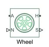
Connection A is the mechanical rotational conserving port for the wheel axle which is given with a PMC. Connection H is the mechanical translational conserving port for the wheel hub through which the thrust developed by the tire is applied to the vehicle. Connection N is a physical signal input port that applies the normal force acting on the tire which connected by the NR port from the vehicle body. The force is considered positive if it acts downwards. Connection S is a physical signal output port that reports the tire slip which is connected to the PS terminator.
Parameters used:
| Parameterize by | Constant Magic Formula coefficients |
| Magic formula B coefficient | 10 |
| Magic formula C coefficient | 1.9 |
| Magic formula D coefficient | 1 |
| Magic formula E coefficient | 0.97 |
c. Shoe Brake:
It represents a brake arranged as two pivoted rigid shoes symmetrically installed inside or outside a drum and operated by one actuator. The actuator force causes the shoes to exert a friction torque on a shaft connected to the drum.
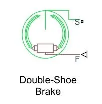
Connection S is a conserving rotational terminal associated with the drum shaft connected with the PMC port with the inertia block at the input. Connection F is a physical signal port representing the force input to the actuator. Positive force creates friction torque that resists shaft rotation. The port F is given input form an inport block with the gain block which represents the barking value to the vehicle's wheel and reduce the speed.
Parameters used:
| Drum radius | 150 | mm |
| Actuator location radius | 100 | mm |
| Pin location radius | 125 | mm |
| Pin location angle | 15 | deg |
| Shoe beginning angle | 5 | deg |
| Shoe span angle | 120 | deg |
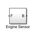
(V) Engine sensor:
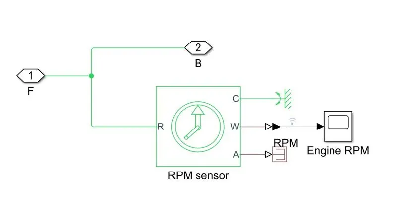
This sensor is us to record the output values from the generic engine to the CVT. The subsystem of this block consists of two PMC port, one Ideal rotational sensor and scope to display the change in the values of speed via increasing or decreasing the throttle. Also, mechanical reference and PS terminator is attache to the connection C and A of the sensor.
fig(x) Subsystem of Engine Sensor
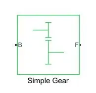
(VI) Simple Gear:
Represents a fixed-ratio gear or gearbox. No inertia or compliance is modelled in this block. You can optionally include gear meshing and viscous bearing losses. Connections B (base) and F (follower) are mechanical rotational conserving ports. Specify the relation between base and follower rotation directions with the Output shaft rotates parameter.
(VII) Solver Configuration: It defines solver settings to use for simulation.
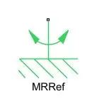
(VIII) Mechanical reference: This block represents a mechanical rotational reference point, that is, a frame or aground. Use it to connect mechanical rotational ports that are rigidly affixed to the frame (ground).
(IX) Goto & From blocks:
Goto blocks are used to send signals to From blocks that have the specified tag and From blocks are used to receive signals from the Goto block with the specified tag If tag visibility is 'scoped', then a Goto Tag Visibility block must be used to define the visibility of the tag. The block icon displays the selected tag name (local tags are enclosed in brackets, [], and scoped tag names are enclosed in braces, {}).
(X) Scope: It display signals generated during simulation.
Steps:
(I) A signal builder block is used to provide the brake and throttle input and the CVT ratio to the system. The output from for the throttle is connected to the generic engine block and the output of CVT gear ratio to the CVT block.
(II) An engine sensor is attached output from the generic engine block. And the output of the engine sensor is attached to the CVT block.
(III) The CVT block takes the inputs from the CVT gear ratio and the engine parameters and provides an output on the wheels. To transfer the CVT power to the wheels, the simple gear block is attached in between them.
(IV) The power output from the simple gear block is attached to the input of vehicle body block where we can check the values of throttling and braking effect and displayed on the scope for the particular effect.
(V) Goto and From block attached to the output of the vehicle body block and scope respectively to display the performance curve when we applied brake or throttle the vehicle.
(2) ATV Model with a dashboard:-
The below figure represents the Simulink model for the BAJA ATV using the CTV for power transmission using a dashboard.
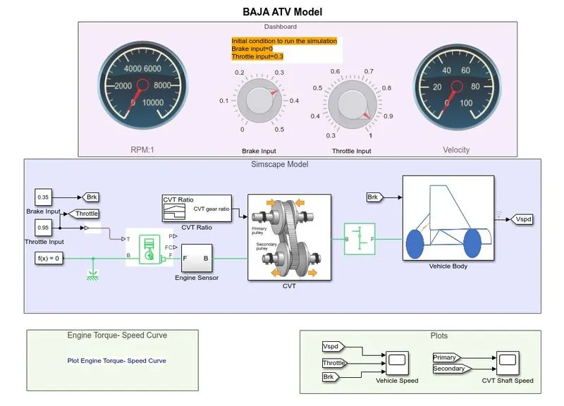
fig(xi) Simulink Layout of AVT model using dashbaord
The process is the same as above, the only change is that instead of the signal builder, we are using a Circular gauge block which acts as a speedometer where values can be displayed from the inputs knob.
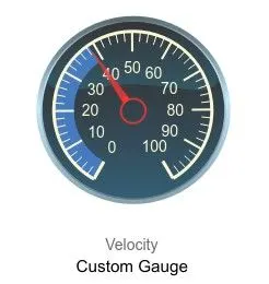
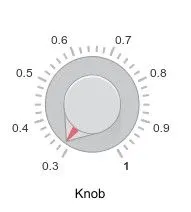
fig(xii) The Simulink block of Custom gauge and a Knob
The knob is used to provide the input values for Brake and throttle where we can set the knob placement as per the required conditions.
Rest the entire process is the same.
Resulted graphs:
The output graphs from default values of brake=0 and throttle =0.3.
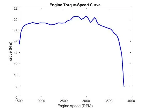
fig(xiii) Torque - Speed Curve
fig(xiv) Vehicle Speed graph
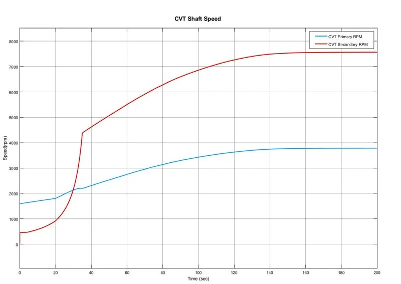
fig(xv) CVT Shaft Speed graph
Observation:
(I) The torque is high at the start as it is required for pickup. But as the speed increases the torque is reduced and for the given input it is `8 N/mm^2`
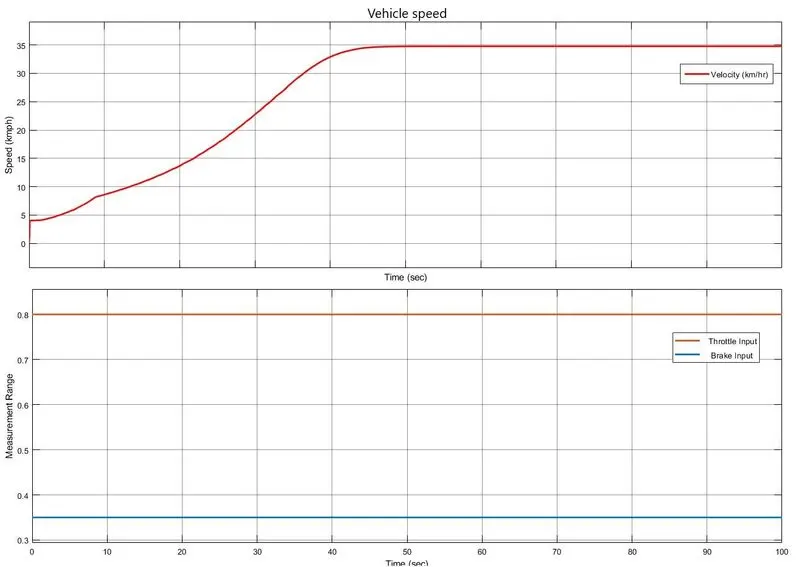
(II) The vehicle speed increases gradually and becomes constant at a certain level as we can see in the velocity speed graph.
(III) The value is '0' at the start for the driving gear which is represented by CVT primary RPM and then a sudden increase in the rpm with less time.
-----------------------------------------------------------------------------------------------------------------------------------------------------------------------------------------
PART 2: Simulink model of ATV with a lookup table
(1) ATV Model without a dashboard:-
The below figure represents the Simulink model for the BAJA ATV using the CTV for power transmission using a lookup table.
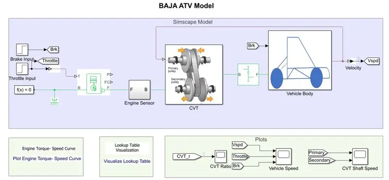
fig(xvi) Simulink model of AVT Model with lookup table
Blocks used:
(I) Lookup Table:
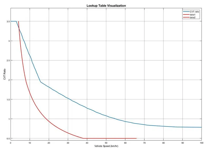
A lookup table is an array of data that maps input values to output values, thereby resembling a mathematical function. If there are a given a set of input values, a lookup operation retrieves the corresponding output values from the table. In other words, a lookup table computes an approximation to some mathematical function y=f(x), given data vectors x and y. We can define the lookup table by specifying a vector of output values parameter as a 1-by-n vector. The lookup table block in Simulink generates an output based on the input values using one of the methods selected from the Look-up method parameter list. If the lookup table does not define the input values, the block estimates the output values based on a nearby table.
In this, we are using the output signal from the vehicle body as the input to the CVT as the CVT gear ratio. It needs to be loaded in the workspace having the file name as Lookuptable_data.mat
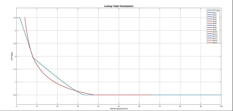
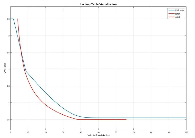
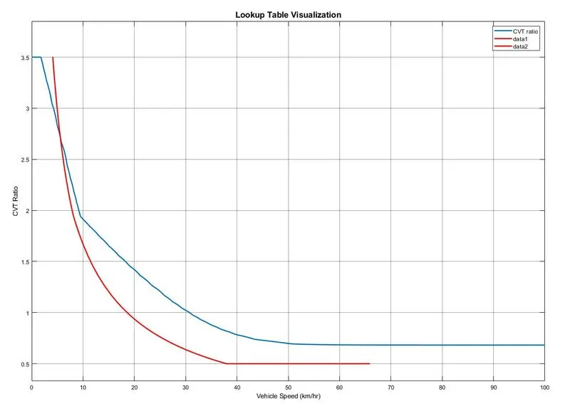
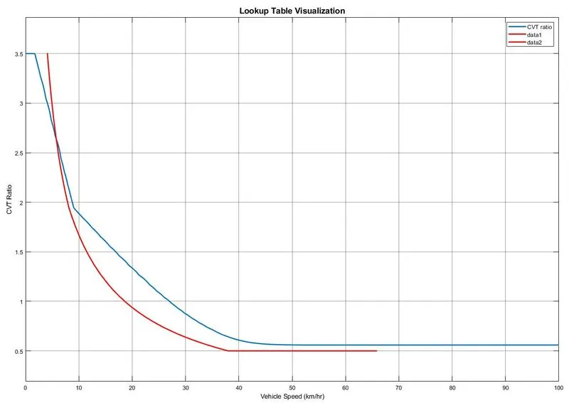
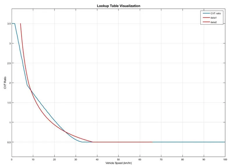
CVT Ratio vs Vehicle Speed:
0-20 kmph, the CVT ratio is constant at 2.3
20-30 kmph, the CVT ratio drops down to 2.03
30-50 kmph, the CVT ratio drops down to 1.8
50 kmph onwards, the CVT ratio is constant at 1.8
(II) Step block: The output is defined in steps.
| Inputs | Brake | Throttle |
| Step time | 35 | 20 |
| Initial value | 0 | 0.3 |
| Final value | 0 | 1 |
| Sample time | 0 | 0 |
Procedure and the working is as the above, the only difference is the lookup table.
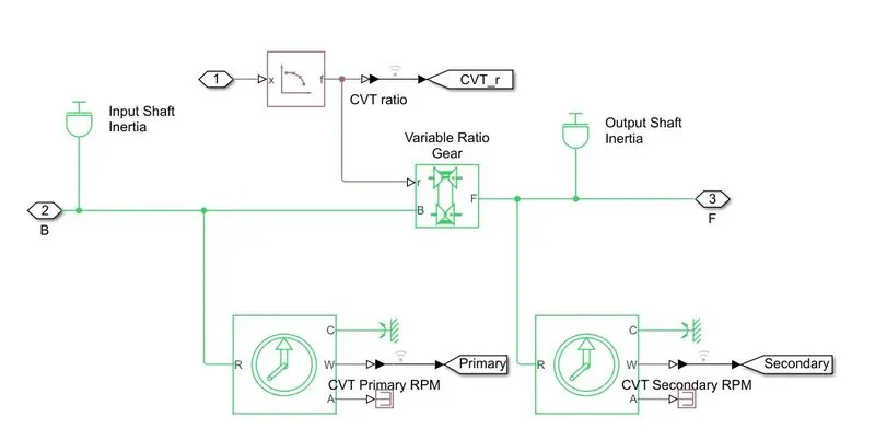
fig(xvii) Subsystem of CVT using Lookup table
(2) ATV Model with a dashboard:-
The below figure represents the Simulink model for the BAJA ATV using the CTV for power transmission using a dashboard along with the lookup table.
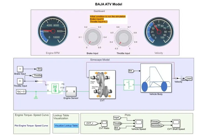
fig(xviii) Simulink model of AVT Model with lookup table
The process is the same as above, the only change is that instead of step input, we are using a Circular gauge block which acts as a speedometer where values can be displayed from the inputs knob.
The knob is used to provide the input values for Brake and throttle where we can set the knob placement as per the required conditions.
Rest the entire process is the same.
Resulted graphs:
The output graphs from default values of brake and throttle.
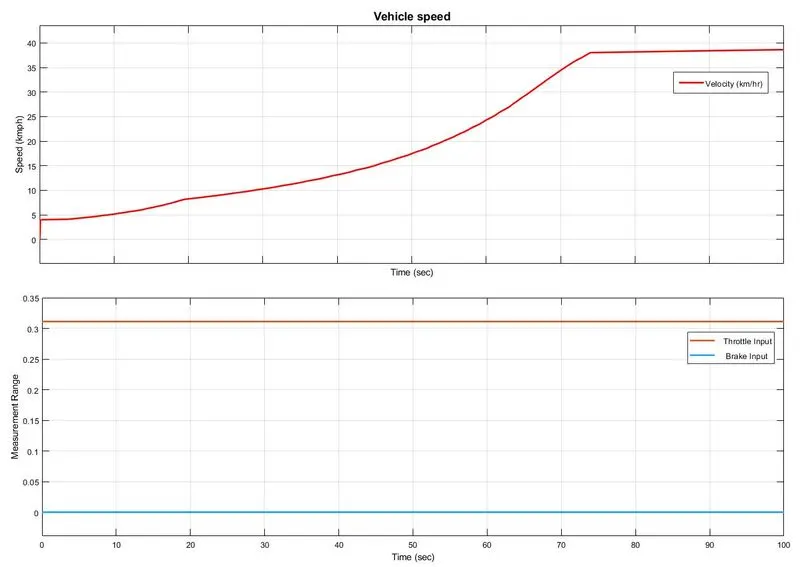
fig(xix) Vehicle Speed graph
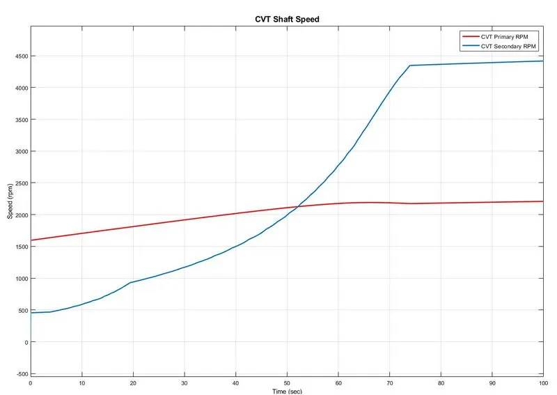
fig(xx) CVT Shaft Speed graph
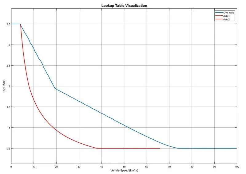
fig(xxi) Lookup table visualization
Observation:
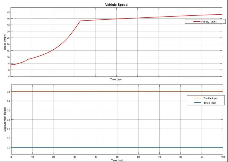
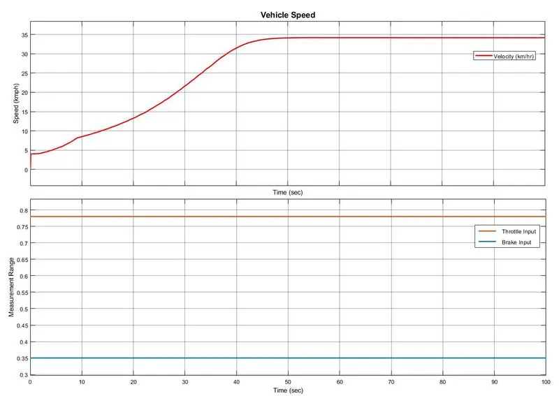
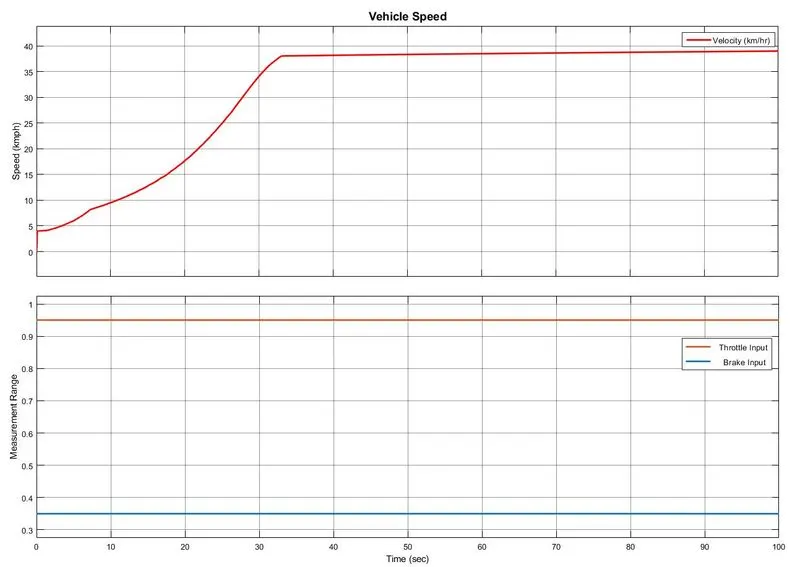
(I) Using the lookup table, the vehicle speed increases gradually and takes longer time to becomes constant at a certain level as we can see in the vehicle speed graph as compared to the previous model.
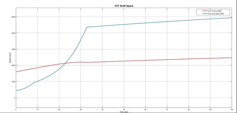
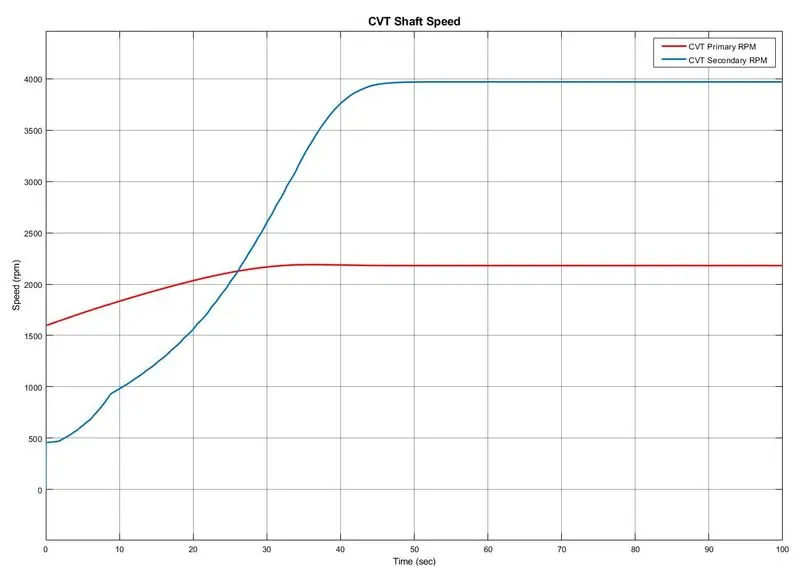
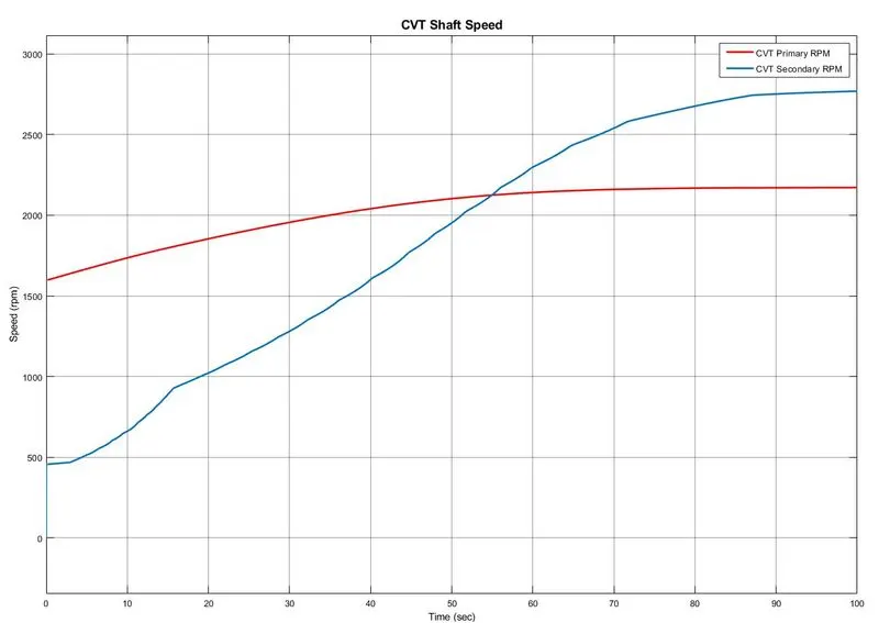
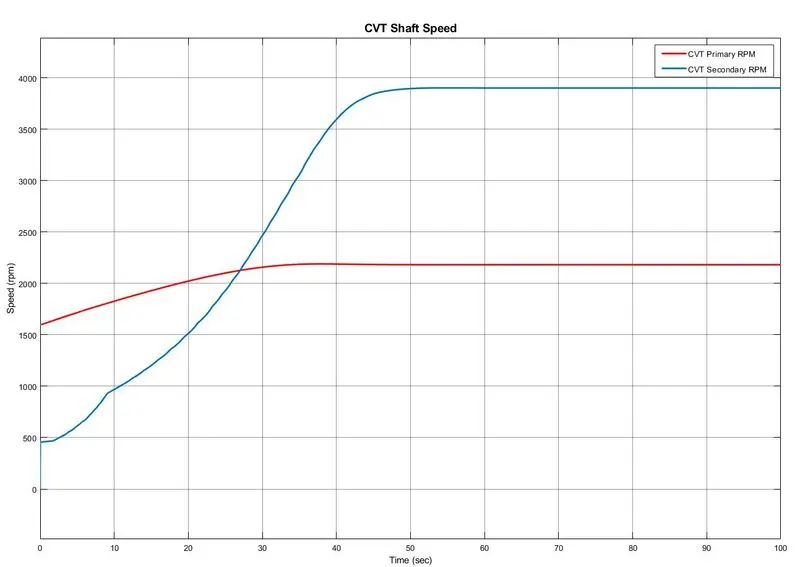
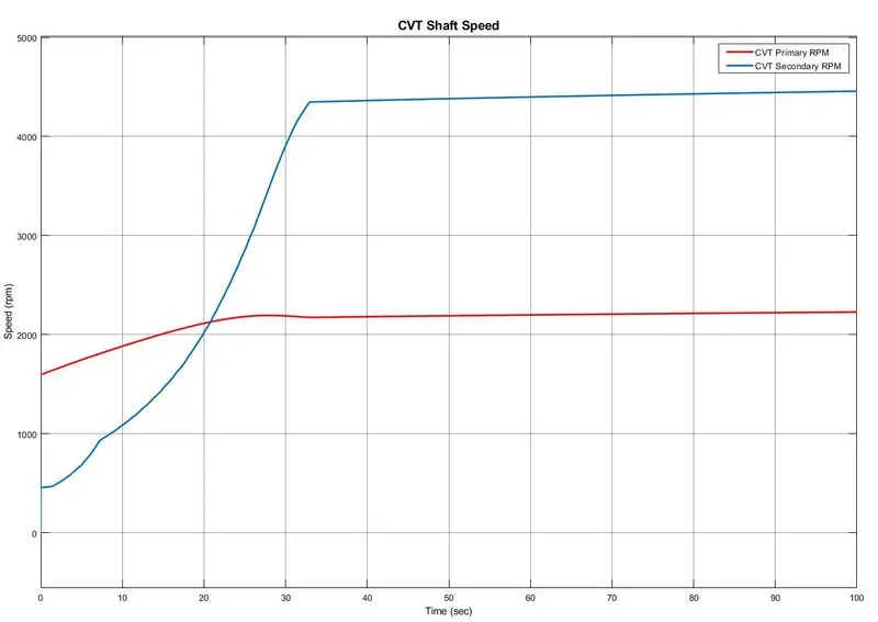
(II) There is a gradual increase in the speed at the secondary gear of the CVT as the initial speed is picked by the driving gear i.e. the primary CVT.
(III) The lookup table graph shows the CVT ratio w.r.t. the output power at the wheel.
-----------------------------------------------------------------------------------------------------------------------------------------------------------------------------------------
TEST CASES:
PART 1: Simulink model of ATV without a lookup table with the dashboard
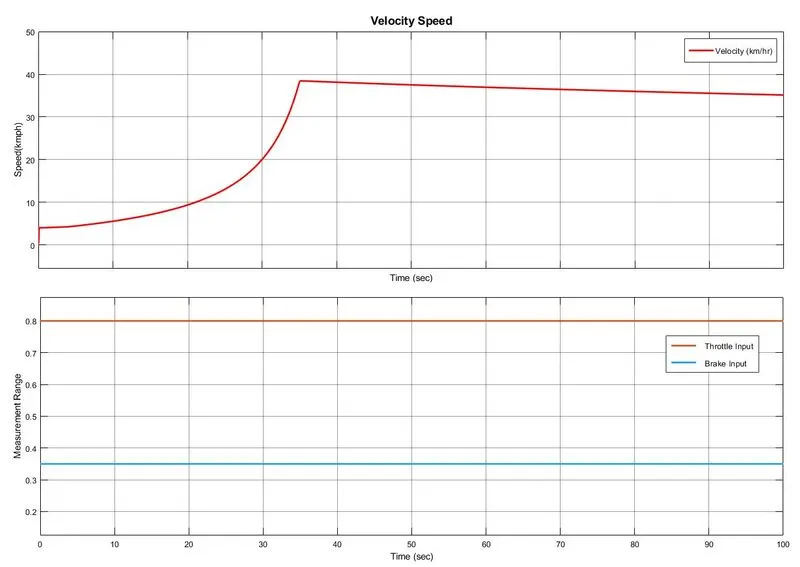
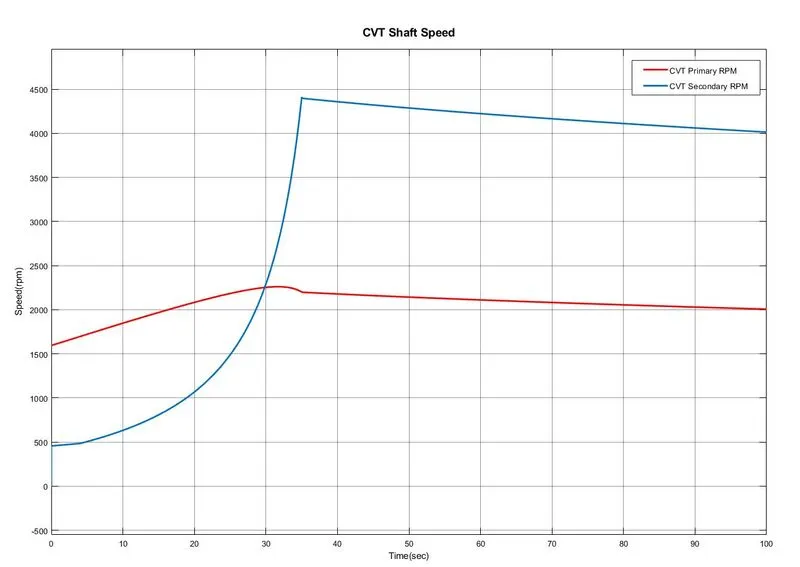
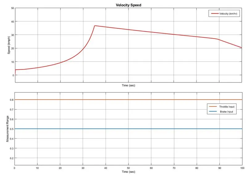
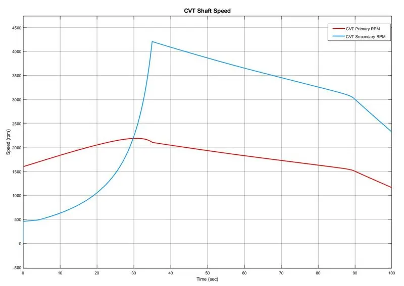
Input#1.1: Change the brake value and throttle is constant.
| Inputs | Brake | Throttle |
| Case 1 | 0.2 | 0.8 |
| Case 2 | 0.35 | 0.8 |
| Case 3 | 0.5 | 0.8 |
Output#1.1:
Case 1:
(I) Vehicle speed:-
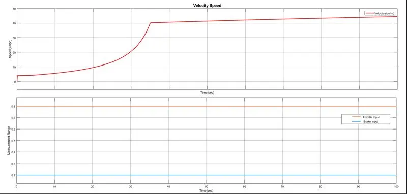
(II) CVT Shaft speed:-
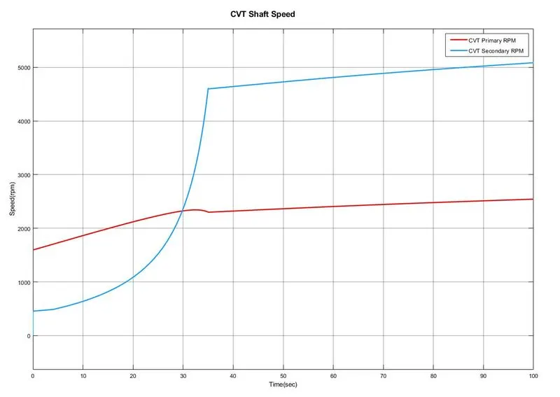
(III) Engine Torque - Speed curve:-
Case 2:
(I) Vehicle speed:-
(II) CVT Shaft speed:-
(III) Engine Torque - Speed curve:-
Case 3:
(I) Vehicle speed:-
(II) CVT Shaft speed:-
(III) Engine Torque - Speed curve:-
Input#1.2: Change the throttle value and brake is constant.
| Inputs | Brake | Throttle |
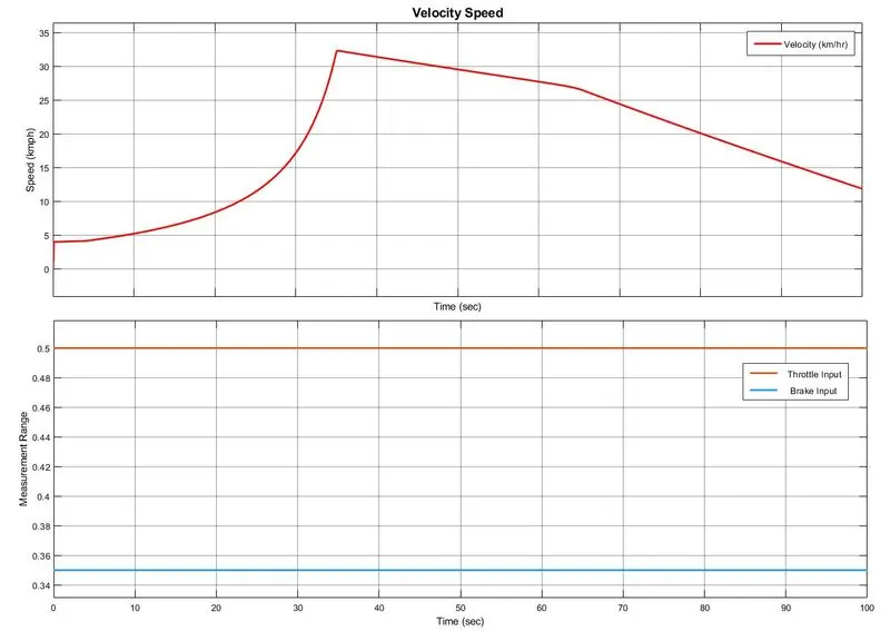
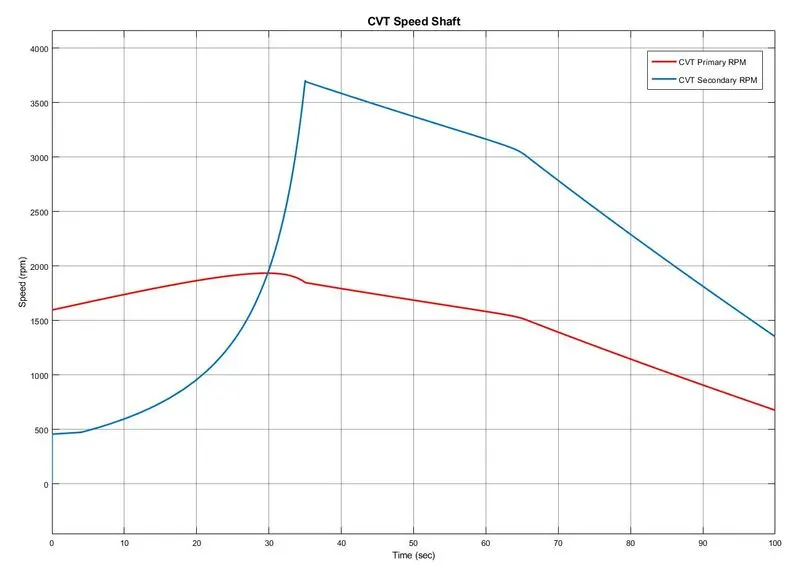
| Case 1 | 0.35 | 0.5 |
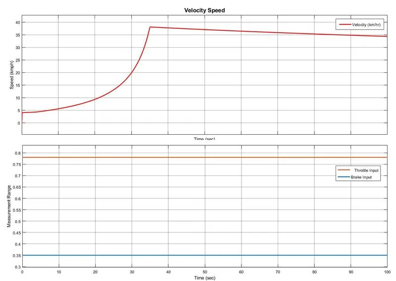
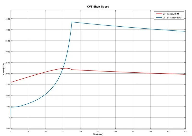
| Case 2 | 0.35 | 0.78 |
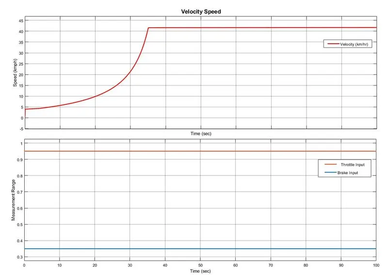
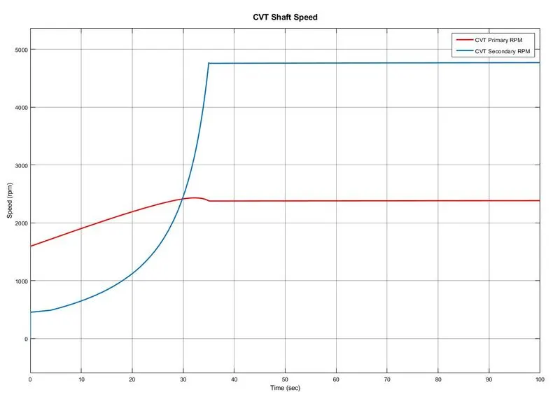
| Case 3 | 0.35 | 0.95 |
Output#1.2:
Case 1:
(I) Vehicle speed:-
(II) CVT Shaft speed:-
(III) Engine Torque - Speed curve:-
Case 2:
(I) Vehicle speed:-
(II) CVT Shaft speed:-
(III) Engine Torque - Speed curve:-
Case 3:
(I) Vehicle speed:-
(II) CVT Shaft speed:-
(III) Engine Torque - Speed curve:-
PART 2: Simulink model of ATV with a lookup table with the dashboard
Input#2.1: Change the brake value and throttle is constant.
| Inputs | Brake | Throttle |
| Case 1 | 0.2 | 0.8 |
| Case 2 | 0.35 | 0.8 |
| Case 3 | 0.5 | 0.8 |
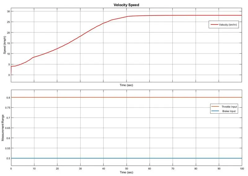
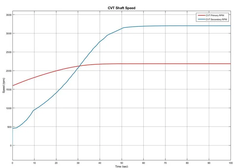
Output#2.1:
Case 1:
(I) Vehicle speed:-
(II) CVT Shaft speed:-
(III) CVT ratio with the look-up table variables:-
Case 2:
(I) Vehicle speed:-
(II) CVT Shaft speed:-
(III) CVT ratio with the look-up table variables:-
Case 3:
(I) Vehicle speed:-
(II) CVT Shaft speed:-
(III) CVT ratio with the look-up table variables:-
Input#2.2: Change the throttle value and brake is constant.
| Inputs | Brake | Throttle |
| Case 1 | 0.35 | 0.5 |
| Case 2 | 0.35 | 0.78 |
| Case 3 | 0.35 | 0.95 |
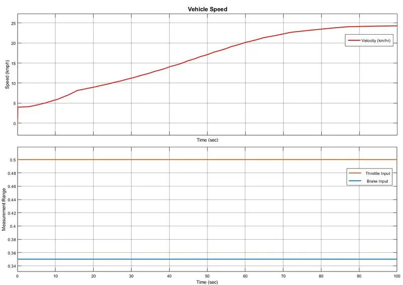
Output#2.2:
Case 1:
(I) Vehicle speed:-
(II) CVT Shaft speed:-
(III)CVT ratio with the look-up table variables:-
Case 2:
(I) Vehicle speed:-
(II) CVT Shaft speed:-
(III) CVT ratio with the look-up table variables:-
Case 3:
(I) Vehicle speed:-
(II) CVT Shaft speed:-
(III) CVT ratio with the look-up table variables:-
Observation:
(I) Base on the same model, we change the values of brake and throttle at the input to get the different behaviour of the vehicle speed, the power output at the CVT shaft speed and the change in the torque-speed curve.
(II) Perform the output graph while keeping the values brake input constant and any test cases with the throttle input constant.
(III) Also, the graphs changes vary when using the lookup table,i.e. taking the output values from the vehicle body and used as the input CVT ratio gear to the CVT system.
-----------------------------------------------------------------------------------------------------------------------------------------------------------------------------------------
CONCLUSION:
(1) Successfully studied and carry out a system-level simulation of an all-terrain vehicle of SAE BAJA.
(2) Observed the vehicle speed, CVT shaft speed and Torque-Speed curve graphs when changing the values of throttle and brake at the input.
(3) The speed becomes constant after certain rpm and decreases when the brakes are applied at different time.
REFERENCE:
https://www.mathworks.com/matlabcentral/fileexchange/70576-baja-all-terrain-vehicle-atv-model