Project 1 - Parsing NASA thermodynamic data

Parsing NASA thermodynamic data

Parsing

Parsing a file means reading in a data stream and building a memory model of the content of that data. This aims at facilitating performing some kind of transformation on the data. Parsing splits a file or other input into pieces of data that can be easily stored or manipulated.

Here we can read the information from any particular text file and we can use the information in programme.

Reading and closing a file

Use ‘fopen’ to open the file, specify the character encoding, and obtain the fileID value. When you finish reading, close the file by calling ‘fclose’(fileID)

OBJECTIVE

Writing a function that extracts the 14 co-efficients from NASA thermodynamic data file and calculates the enthalpy, entropy and specific heats for all the species in the data file.

Formula used to Calculate CP,H,S

The FIRST 7 coefficients are HIGH-temperature coefficients and the SECOND 7 coefficients are LOW-temperature coefficients.

Also use the LOCAL TEMPERATURE RANGES which is unique for each individual species, not the GLOBAL TEMPERATURE RANGE.

Code Used

FOPEN

It opens file, or obtain information about open files.

Syntax

fileid=fopen(filename)

fgetl

It returns an output that displays in one line, while fgets returns an output that includes the newline character and, therefore, displays it in two lines.

Syntax

line = fgetl( fileID )

strsplit

Split string or character vector at specified delimiter.

Syntax

c=strsplit(ste,delimeter)

str2double

It converts the text in str to double precision values. str contains text that represents real or complex numeric values.

mkdir

It creates folderName in parentFolder . If parentFolder does not exist, MATLAB attempts to create it.

Syntax

mkdir parentfolder folder name

Fclose

It closes file.

Syntax

fileid=fclose(filename)

DATA FILE LINK

https://drive.google.com/file/d/1AikCHDlz9s_fu8whE81qee_GD4AyYpCP/view?usp=sharing

MATLAB CODE FOR FILE PARSING

clear all
close all
clc

f1=fopen('THERMO.dat','r')% Read the file
fgetl(f1) %Read the 1st line
global_temp=fgetl(f1)
Temp=strsplit(global_temp,' ')%delimeter for space
global_min_temp=str2num(Temp{2})
global_mid_temp=str2num(Temp{3})
global_high_temp=str2num(Temp{4})

%skip 3 lines
for n=1:3
    fgetl(f1)
end

for j=1:53 % FOR ITRATION OF ALL SPECIES
local_temp=fgetl(f1)
X=strsplit(local_temp,' ') %split the string
species_name=X{1}
L=length(X)
local_min_temp=str2num(X{L-3})
local_high_temp=str2num(X{L-2})
local_mid_temp=str2num(X{L-1})
% LOcating The Coeffeicent
%Calling 1st Line
Line_1=fgetl(f1)
a=findstr(Line_1,'E')%finding the position of E
a1=str2double(Line_1(1:a(1)+3));
a2=str2double(Line_1(a(1)+4:a(2)+3));
a3=str2double(Line_1(a(2)+4:a(3)+3));
a4=str2double(Line_1(a(3)+4:a(4)+3));
a5=str2double(Line_1(a(4)+4:a(5)+3));

%calling 2nd Line
Line_2=fgetl(f1)
b=findstr(Line_2,'E')
a6=str2double(Line_2(1:b(1)+3)); % convert the string to number
a7=str2double(Line_2(b(1)+4:b(2)+3));
a8=str2double(Line_2(b(2)+4:b(3)+3));
a9=str2double(Line_2(b(3)+4:b(4)+3));
a10=str2double(Line_2(b(4)+4:b(5)+3));
%Calling The 3rd Line
Line_3=fgetl(f1)
c=findstr(Line_3,'E')
a11=str2double(Line_3(1:c(1)+3));
a12=str2double(Line_3(c(1)+5:c(2)+3));
a13=str2double(Line_3(c(2)+4:c(3)+3));
a14=str2double(Line_3(c(3)+4:c(4)+3));

%setting Temp range 
mkdir(['C:\Users\Admin\Desktop\nasa\',species_name])
T=linspace(local_min_temp,local_high_temp,1000);
R=8.314
for i=1:length(T)
    if T(i)>local_mid_temp
        CP(i)=(a1+a2*T(i)+a3*T(i)^2+a4*T(i)^3+a5*T(i)^4)*R;
        H(i)=((a1+(a2*T(i)/2)+(a3*T(i)^2)/3)+((a4*T(i)^3)/4)+((a5*T(i)^4)/5)+(a6/T(i)))*(R*T(i));
        S(i)=(a1*log(T(i))+a2*T(i)+(a3*T(i)^2)/2+(a4*T(i)^3)/3+(a5*T(i)^4)/4+a7)*R;
    else 
        CP(i)=((a8+a9*T(i))+(a10*T(i)^2)+(a11*T(i)^3)+(a12*T(i)^4))*R;
        H(i)=(a8+(a9*T(i))/2+(a10*T(i)^2)/3+(a11*T(i)^3)/4+(a12*T(i)^4)/5+a13/T(i))*(R*T(i));
        S(i)=(a8*log(T(i))+a9*T(i)+(a10*T(i)^2)/2+(a11*T(i)^3)/3+(a12*T(i)^4)/4+a14)*R;
    end
end

%PLOTTING THE GRAPH
figure(1)
plot(T,CP,'linewidth',3,'color','r')
grid on
title(species_name)
xlabel('T')
ylabel('CP')
figure(2)
plot(T,H,'linewidth',3,'color','r')
grid on
title(species_name)
xlabel('T')
ylabel('H')
figure(3)
plot(T,S,'linewidth',3,'color','r')
grid on
title(species_name)
xlabel('T')
ylabel('S')

%SAVING THE FILE
cd(['C:\Users\Admin\Desktop\nasa\',species_name])
saveas(1,'CP.jpg')
saveas(2,'H.jpg')
saveas(3,'S.jpg')

   %calulation of molecular weight
 elements={'O','H','C','N','A'};%common element for all species
 atomic_weight=[15.999 1.0079 12.0107 14.0067 39.948];
 mol_mass=0;
 for i=1:length(species_name)
     for j=1:length(elements)
         if strcmp(species_name(i),elements(j))%it compairs the species with elemnts if it is same the it read the value 
             mol_mass=mol_mass+atomic_weight(j);
             place=j;
         end
     end
     n=str2num(species_name(i));
     if n>1
         mol_mass=mol_mass+atomic_weight(place)*(n-1);
     end
     
             
 end
 
sprintf('Molecular Weight of %s:%f u',species_name,mol_mass)

 
 
end
fclose(f1)

OUTPUT

O2

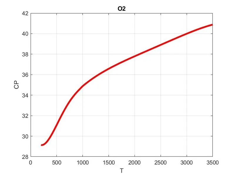
CP VS T

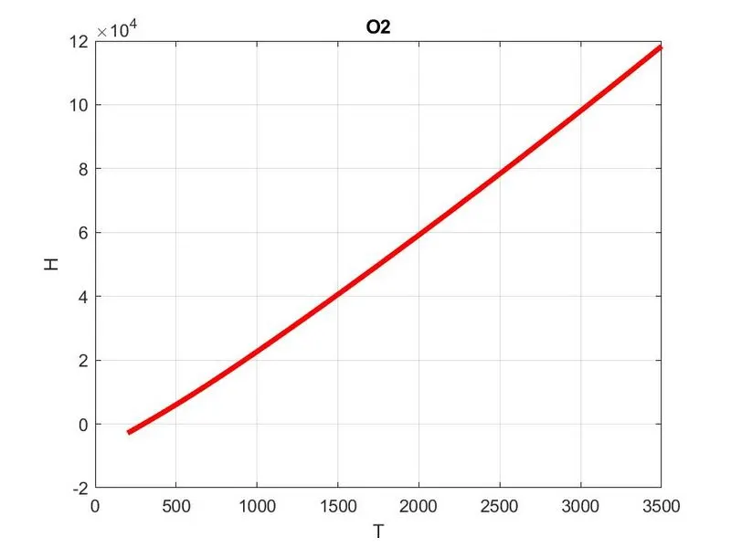
H VS T

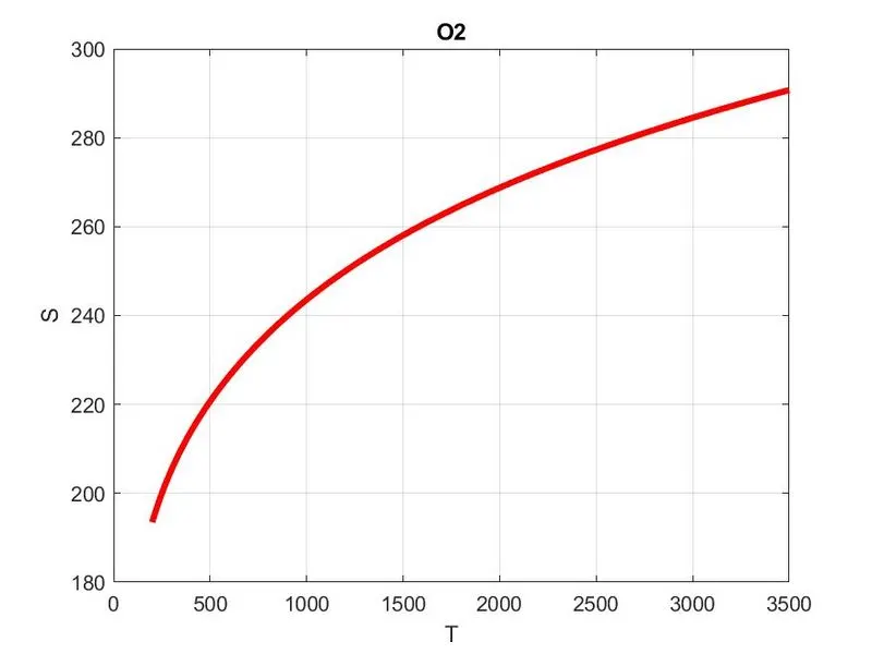
S VS T

MOLECULAR WEIGNT OF O2

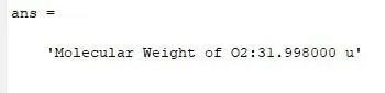
N2

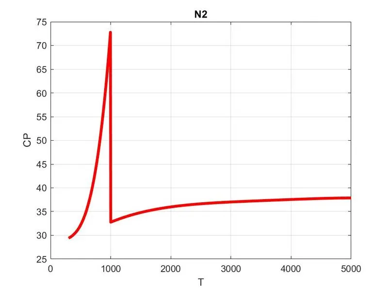
CP VS T

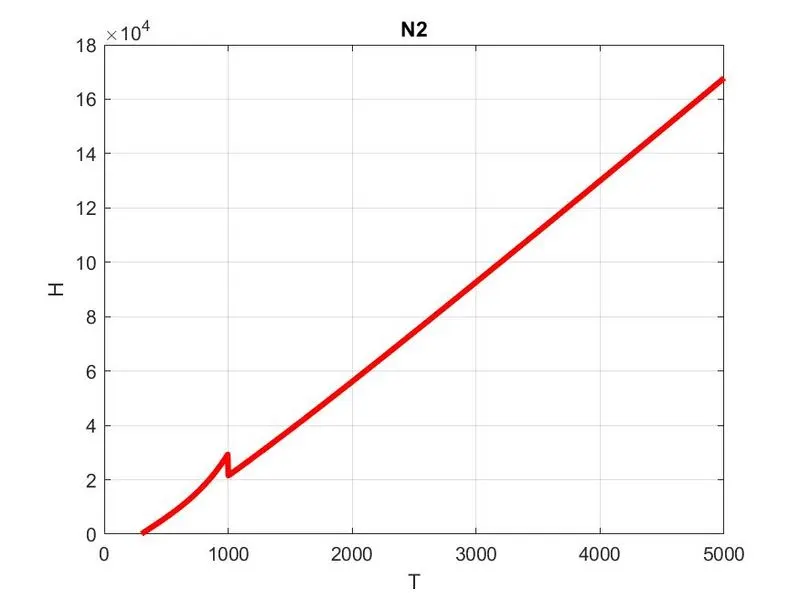
H VS T

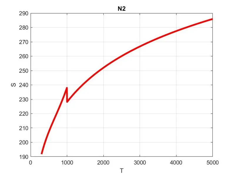
S VS T

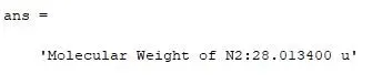
MOLECULAR WEIGNT OF N2

CO2

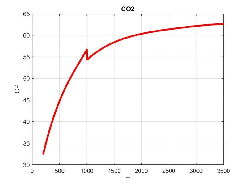
CP VS T

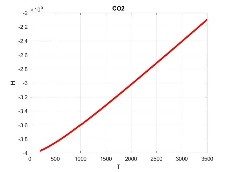
H VS T

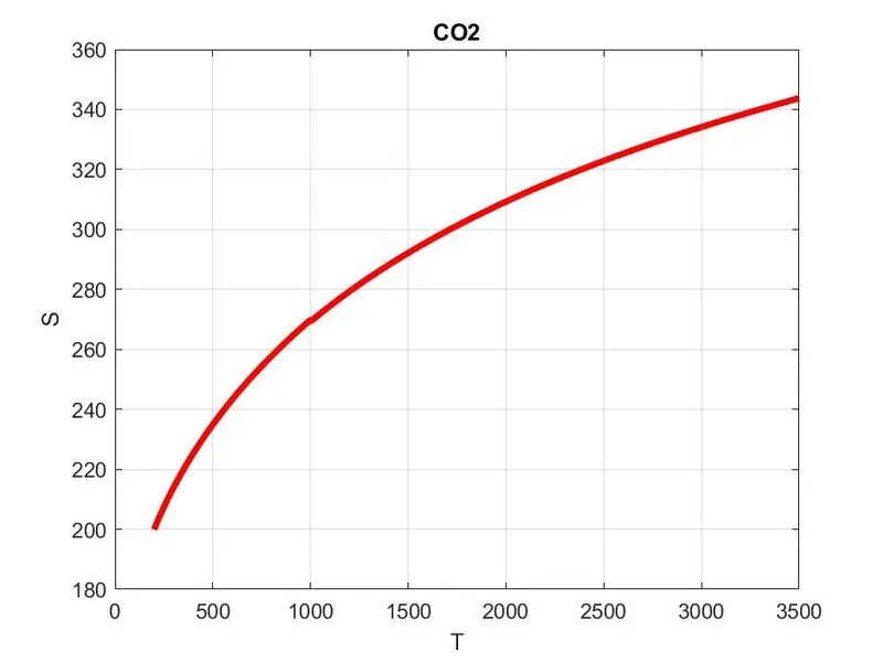
S VS T

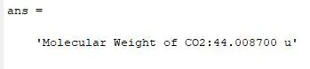
MOLECULAR WEIGNT OF CO2

FOLDER FOR ALL SPECIES

CONCLUSION

Here we sucessefully parsing the data file and we obeserve how themodynamic properties are change with respect to tempertaure.