Forward Energy Based Model for Fuel Consumption in a Conventional Vehicle by using Matlab and Simulink

Objectives:

• To build a Forward energy based fuel comsumption model for conventional vehicle
• To estimate the fuel economy number for different drive cycle(UDDS and HWFET)
• To find out working region of an engine for UDDS and HWFET drive cycle.
• To observe the speed of various component with respect to time

Keywords:Forward Based Model,UDDS, HWFET, Fuel economy.

1 Introduction

A forward facing vehicle features a driver model provides torque demand which is in form of desired brake torque and engine torque which is required to meet the speed demand from the drive cycle. A driver model consits of one or more proportinal Inetegrator (PI) block to meet the torque demand with respect to the speed of the drive cycle.The engine torque is transmitted to the transmission and ends as a torque applied to the wheel. This wheel torque is exerted to the vehicle mass via force acting on the tyre contact patch. The vehicle speed which is obtained after overcoming all the resistance force is propragated back to the driver model. And based on the speed trace of the drive cycle and actual vehicle speed , again torque demand and brake torque demand is created, Brake torque is directly fed to the wheel. Figure 1 shows the forward facing model . As in the real world driver, driver model has to minimize the error margin.Forward facing model also provides the understanding regarding the drivability and captures the limitation of physical system. It also provide the easy integration of control system. For forward facing model simulation has to run through a smaller time step as it have the multiple equation to compute out the vehicle speed which result in longer simulation time. The driver model can be re tuned to maximise the performance of the system in the area related to fuel economy and longitudinal accleration[1].

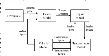
Figure1: Forward Based Model

2.Model Development

The model for forward energy based fuel consumption consists for following:

1. Driver
2. Controller
3. Powertrain

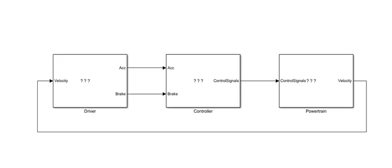
Figure2: Forward energy based Model

2.1 Driver Model

Driver model is made up of Proportional intergrator (PI) controller, Drive crycle etc. PI controller check the difference between the vehicle speed and drive cycle trace speed and based on the error it provides the position of brake and acclerator pedal which eventually becomes a torque request to the powertrain block.Gain for proportional and integrator block is taken as 50 and 5 respectively. To stopping the simulation automatically it also contains an extra arrangement where end velocity and end time are feed into the AND block. If conditions satisfies the simulation stops. Figure 3 shows the detail about driver model used for this project.

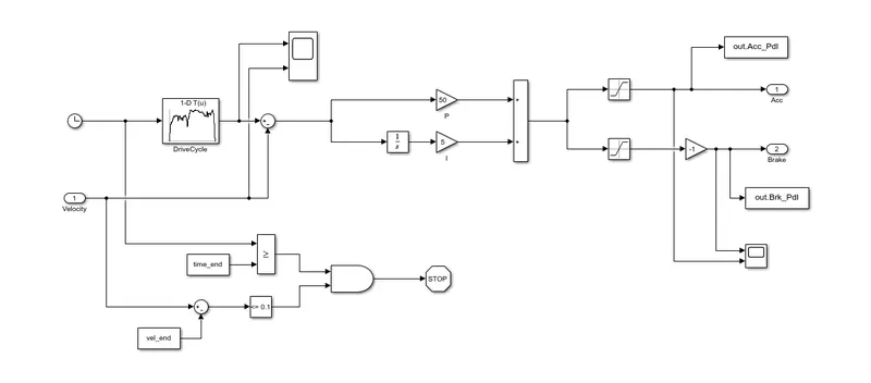
Figure3: Driver Model for the project

2.2 Controller Model

From the controller model, torqe request for the brake and engine is send out to the powertrain. And based on the vehicle speed and throttle input Gear command is also fetch to the powertrain. Further, Controller is divided into 3 secton which are:

1. Engine Control block
2. Transmission Control block
3. Brake Control block

Signal from the all the above mentioned control block is merged together by using the bus creator and send it to the powertrain as a control signal. The detailed view of controller model is shown in figure 4.

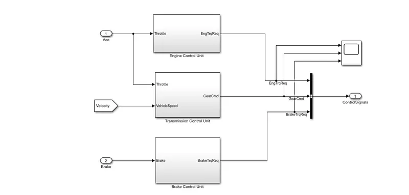
Figure3: Controller block showing different control unit

2.2.1 Engine Control Unit

In engine control unit, based on the engine speed maximum and minimum torque is estimated from the 1D look up table. To simulate for the engine idling a seprated controller is made which provides the throttle opening for idle speed. In the engine idle controller, engine speed is compared with the idling speed of engine and based on the error a PI controller gives the throttle opening during idling. The gain for proportional and integrator block is 1 and 0.01 respectively.Figure 4 shows the engine idle controller. The throttle position from the driver model is added with the idle throttle, which is than multiplied with the net torque , which gives the torque request for the engine. Figure 5 shows the engine control unit for the project.

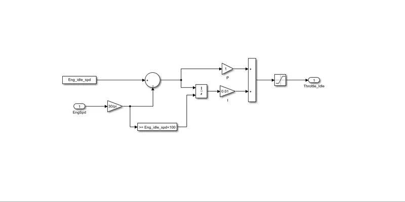
Figure 4: Engine Idle Controller

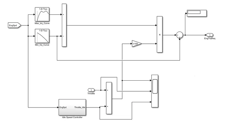
Figure5: Engine Control unit used for the project

2.2.2 Transmission Control Unit

In transmission control unit, throttle opening and vehicle speed is feed into controller and based on the input vehicle gear command is generated. Based on the transmission shift logic which is shown in figure 6 gear command is generated.

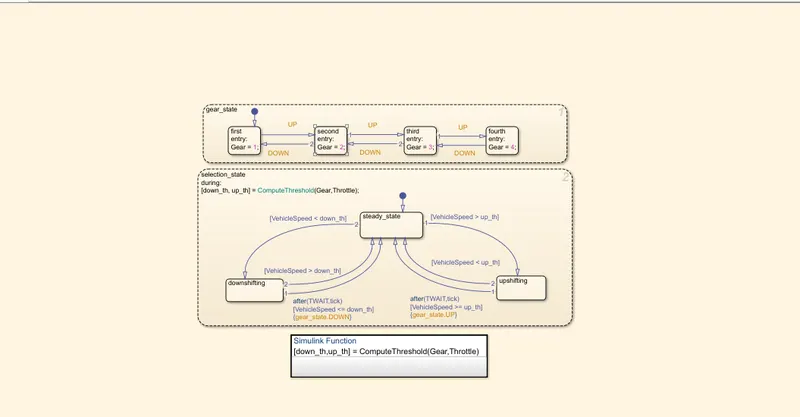
Figure 6: Transmission shift logic

2.2.3 Brake Control Unit

In brake control, brake position from the driver model is fed and brake torque request is generated. The detail of brake control unit is shown in figure 7

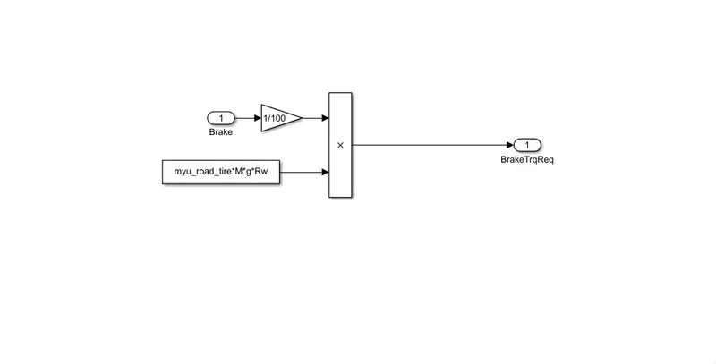
Figure 7; Brake control Unit

2.3 Powertrain Block

In powertrain block, control signal from controller is fed into it and based on the control signal vehicle performs. It also contains the bus selector which splits the control signal as torque request, brake question and gear command. This signal are fed into different sub block according to their uses. The powertrain block consits of following subblock which is shown in figure 8.

1. Engine
2. Transmission
3. Differential
4. Wheels and
5. Vehicle Dynamics

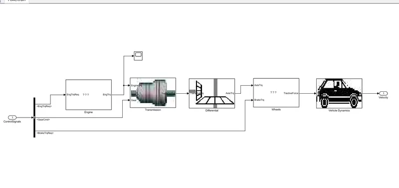
Figure8: Powertrain block used for the project

2.3.1 Engine

In engine subblock, torque request from the controller is supplied as a input signal and based on the torque request saturation dynamic block limit the value of torque within maximum and minimum torque of an engine. A 2D look up table is used to find the fuel consumption of an engine when it is function at a certain speed and torque. The output of an engine subblock is the engine torque which is transmitted to the transmission unit. Figure 9 shows the engine subblock.

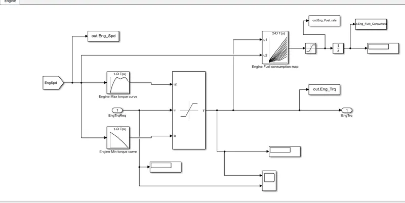
Figure 8: Engine subBlock

The fuel consumed is determined as a function of engine speed and torque,i.e.

`dot(mf)=Fun(Es,T)` where Es is engine speed , T is Engine Torque , mf is instantaneous fuel consumption.

The total fuel consumed=`mf=intdot(mf)dt`

2.3.2 Transmission Block

In transmission block, gear command from controller section and engine torque from engine subblok is send as a input signal . It also contains the subblock inside it for torque converter. In torque converter block based on the engine dynamic and engine torque, input speed to the torque converter is calculated. By using formula as mentioned below different parameter for torque converter is computed. Figure 9 shows the torque converter block. In transmission block,based on the gear command , a gear ratio is selected form 1D look up table which is multiplied with output from the torque converter block(transmission In speed) to get the output speed of a transmission system. Based on the working condition, there may be positive and negative output. Figure 10 shows the transmission system block.

Equation Used:

1. Speed ratio, `SR=(wt)/(wp)`
2. Torque ratio, `TR=(Tt)/(Tp`
3. Capacity factor, `K=(wp)/sqrt(Tp)`

where, wt, wp is the speed of pump and turbine of torque converter while Tp and Tt is the torque of pump and turbine.

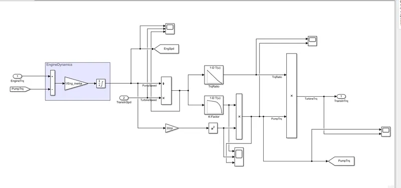
Figure 9: Torque converter model in simulink

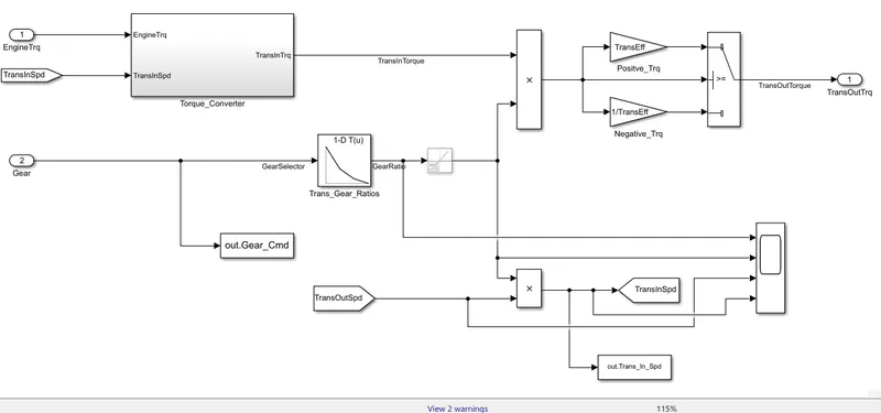
Figure 10: Transmission system Block

2.3.3 Differential

In differential block, output torque from the transmission is fed in as a input which is multiplied with final drive ratio of vehicle and gives the axle torque. Figure 11 shows the differential subblock.

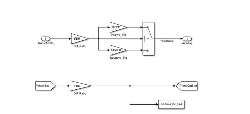
Figure 11: Differential subblock

2.3.4 Wheels

In wheel brake troque request from the control and axle torque from the differential is fed as a input and based on the wheel radius tractive force is calcultated. Figure 12 shows the subblock for the wheel.

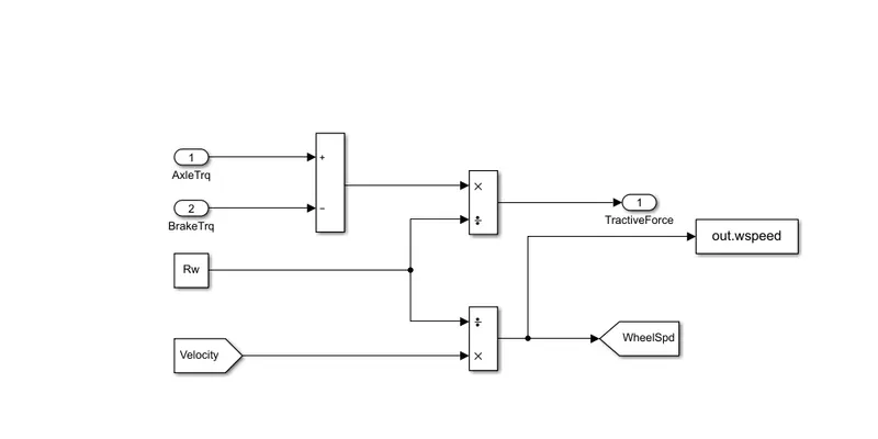
Figure 12: Wheels subblock

2.3.5 Vehicle Dynamic

In vehicle dynamic block the tractive force from the wheel is taken as input. The total resistance force(gradient, Drag,Friction) force or road load is calculated by using below mentioned formula. The road load is subtracted from the tractive force which gives the accleration force. By intergrating accleration force as per our requirement velocity and distance travelled is computed. Figure 13 shows the vehicle dynamic used in this project.

Equation used:

1. Friction force(Road friction),`F_r=Cr.M.gcostheta`
2. Gradient force,`F_g=Mgsintheta`
3. Drag force,`F_d=1/2rhoA_fC_dv^2`
4. Road load,`F_(load)=F_r+F_g+F_d`
5. Accleration,`a=(F_(tractive)-F_(load))/M`
6. Velocity,`v=intadt`
7. Distance,`S=intvdt`

where, Cr is rolling resstance coefficient, M is the mass of vehicle, `theta` is the angle of inclination,g is accleration due to gravity,Af is the vehicle frontal area, Cd is the drag coefficient,`F_(tractive)` is the tractive force,`rho` is the density of air

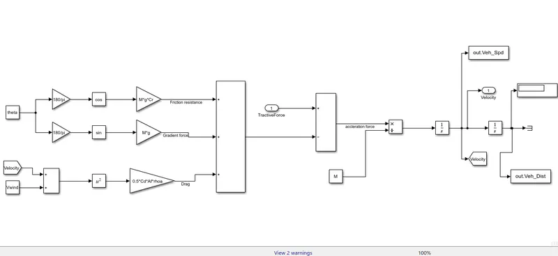
Figure 13: Vehicle dynamic block used for the project.

3. Matlab Code

3.1 Matlab Initilization Script:

For UDDS(Urban Dyanamometer Driving Schedule) cycle , drive cycle select value of 1 is selected while for HWFET(Highway Fuel Economy Test) ,drive cycle select value of 2 is selected.

%% Vehicle Parameters
M = 1500;       % Vehicle weight [kg]
Cr = 0.015;     % Rolling resistance coefficient
Rw = 0.35;      % Rolling radius [m]
Cd = 0.33;      % Drag coefficient
Af = 2;         % Frontal area [m2]
rhoa = 1.225;   % Air density [kg/m3]
Vwind = 0;      % Wind velocity [kmph]
g = 9.81;       % Gravitational acceleration [m/s2]
theta = 0;      % Slope [deg]
myu_road_tire = 1; % Coefficient of friction between tire - road interface

%% Powertrain Parameters 
FDR = 3.73;                         % Final Drive Ratio / Diff Ratio
DiffEff = 0.99;                     % Differential efficiency (assumed independent of operating conditions)

NumGear = 4;                        % Number of gears in transmission
TransGear = [1:NumGear];            % Transmission Gears
TransRatio = [3.06, 1.62, 1, 0.7];  % Corresponding Transmission ratios
TransEff = 0.90;                    % Transmission efficiency (assumed independent of operating conditions)

TC_SR = [0, .5, .6, .7, .8, .87, .92, .94, .96, .97, 1];   % Torque Converter Speed Ratio (Matlab default) -> TurbSpd/PumpSpd  
TC_TR = [2.232, 1.5462, 1.4058, 1.2746, 1.1528, 1.0732, 1.0192, 1, 1, 1, 1];   % Torque Converter Torque Ratio (Matlab default) -> TurbTrq/PumpTrq
TC_Cf = 1e-4 * [.72558, .66322, .63463, .59042, .51331, .4144, .29287, .22444, .12186, .04386, 0]; % Torque Converter Capacity Factor (Matlab default) -> PumpTrq/PumpSpd^2 [Nm/rpm^2]

load Vehicle_Data/Engine_data_1_9L_Saturn_95kW
load Vehicle_Data/Trans_Shift_map

%% Driver Parameters
Kp = 10;                    % P gain for driver PI model
Ki = 1;                     % I gain for driver PI model
Drive_Cycle_Select = 1;     % Drive cycle selection

% Drive cycle values in m/s

if Drive_Cycle_Select == 1
    load DriveCycles/UDDS;
    
elseif Drive_Cycle_Select == 2
    load DriveCycles/HWFET;
    
elseif Drive_Cycle_Select == 3
    load DriveCycles/FTP;
    
elseif Drive_Cycle_Select == 4
    load DriveCycles/US06;
    
elseif Drive_Cycle_Select == 5
    load DriveCycles/NEDC;
    
elseif Drive_Cycle_Select == 6
    load DriveCycles/WLTP;
 
end

time_end = cyc_time(end);
vel_end = cyc_vel(end);

3.2 Matlab Post Processing Script:

%%Extracting data from simulink simulation

Time=out.tout;  %Extracting time
A_pedal=out.Acc_Pdl;  %Acclerator pedal position
B_pedal=out.Brk_Pdl; %Brake pedal position
Ef=out.Eng_Fuel_Consumption; %Fuel consumption data
Es=out.Eng_Spd;  %Engine Speed data
Et=out.Eng_Trq; %Engine Torque data
Gc=out.Gear_Cmd; %Gear command data
Tin=out.Trans_In_Spd*30/pi; %Transmission In speed
Tout=out.Trans_Out_Spd*30/pi; %Transmission Out speed
Dis=out.Veh_Dist; %distance travel during drive 
V=out.Veh_Spd; %Vehicle speed
Fu=out.Eng_Fuel_rate; %Fuel supply to the engine
Ws=out.wspeed; %Vehicle wheel Speed
Ws=Ws.Data(:,1);
Ws=Ws*30/pi;
%%Since some of the above mention varible are in double time series so only
%%extracing data which are only required

Es=Es.Data(:,1)*30/pi;  %Extracting data and changing it to rpm
Et=Et.Data(:,1); %Torque in Nm
Dis=Dis.Data(:,1)/1000;  % changing distance to Km
V=V.Data(:,1); %chaning m/s to km/hr
Ef=Ef.Data(:,1);
Fu=Fu.Data(:,1);

%%Calculating kmpl for the drive cycle
Pw=(Et.*Es*pi/30)/1000;  %Power in KW
rho_p=0.7197; %density of petrol
T_dis=Dis(end); %Total distance in Km
T_fuel=Ef(end); %Total Fuel consumed
Vol=(T_fuel/1000)/rho_p;  %Total litre of fuel 
Milage=T_dis/Vol;

%%Plotting Engine, Transmission and Wheel Speed with respect to time
figure(1)
subplot(3,1,1)
title('Speed of Different component with respect ot Time');
hold
plot(Time,Es); %Plotting Engine speed with respect to time
xlabel('Time in Seconds');
ylabel('Engine Speed in RPM');

subplot(3,1,2)
plot(Time,Tin,'Displayname','Transmission Input Speed');
hold
plot(Time,Tout,'Displayname','Transmissin Output Speed');
xlabel('Time in Seconds');
ylabel('Transmission Speed in RPM');
legend

subplot(3,1,3)
plot(Time,Ws);
xlabel('Time in Seconds');
ylabel('Wheel Speed in RPM');
hold off

%Plotting Engine Torque, Power, Fuel rate and Fuel consumption
figure(2)
title('Engine Behavior with respect to Time');
hold
subplot(2,2,1)
plot(Time,Et);
xlabel('Time in second');
ylabel('Engine Torque N-m');

subplot(2,2,2)
plot(Time,Pw);
xlabel('Time in second');
ylabel('Power in KW')

subplot(2,2,3)
plot(Time,Fu);
xlabel('Time in second');
ylabel('Fuel consumption in gm/s');

subplot(2,2,4)
plot(Time,Ef);
xlabel('Time in Second');
ylabel('Total fuel(gm) consumed in t second');
hold off

%Plotting accleration, brake,gear command, real vs desired speed and
%distance with respect to time

figure(3)
subplot(2,2,1)
plot(Time,A_pedal,'Displayname','Acclrn press');
hold
plot(Time,B_pedal,'Displayname','Brake Press');
xlabel('Time in second');
ylabel('Percentage %');
legend

subplot(2,2,2)
plot(Time,Gc);
xlabel('Time in second');
ylabel('Gear number');

subplot(2,2,3)
plot(Time,Dis);
xlabel('Time in second');
ylabel('Distance in Km');

subplot(2,2,4)
plot(cyc_time,cyc_vel,'Displayname','Desired Speed');
hold on
plot(Time,V,'Displayname','Actual Speed');
xlabel('Time in Second');
ylabel('Velocity in m/s');
legend
hold off

%% Plotting engine operating points on engine fuel map
figure(4);
hold on
title('Engine Operating Points','fontsize',12);
p1=plot(Eng_map_spd*30/pi,Eng_max_trq,'linewidth',2,'color','r');
p2=line([Eng_map_spd(end)*30/pi Eng_map_spd(end)*30/pi],[0 Eng_max_trq(end)]);
set(p2,'linewidth',1,'linestyle','--','color','k');
p3=line([Eng_map_spd(1)*30/pi Eng_map_spd(1)*30/pi],[0 Eng_max_trq(1)]);
set(p3,'linewidth',1,'linestyle','--','color','k');
[c,h] = contour(Eng_map_spd'*30/pi,Eng_map_trq,Eng_fuel_map');
clabel(c,h);
xlabel('Engine Speed [rpm]');
ylabel('Engine Torque [Nm]');

% figure(5)
title('Engine Fuel Consumption Map [g/s]');
p4 = plot(Es,Et,'.','color','k');
legend([p1 p4],{'Max Curve','Operating Points'});
axis([Eng_map_spd(1)*30/pi Eng_map_spd(end)*30/pi 0 Eng_map_trq(end)]);
hold off

%plotting drive cycle
figure(6)
plot(cyc_time,cyc_vel);
xlabel('Time in Second');
ylabel('Velocity in m/s');

4. Result

The model is run for the different drive cycle and following results are made:

4.1 Fuel Economy

For both driver cycle forward energy based model has been simulated. The vehicle travels a total of around 16.5 km for the HWFET cycle and around 12 km for the UDDS cycle. The total amount of fuel consumed for the HWFET cycle was around 1 litre and for UDDS cycle was 0.85 litre. The milage obtained for UDDS cycle was around 14.10 Kmpl while for HWFET it was around 16.5Kmpl. Figure 14 shows the comparision between UDDS and HWFET cycle in terms of fuel economy.

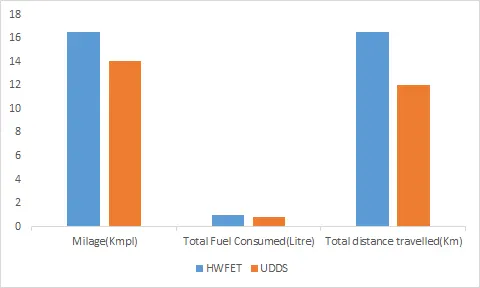
Figure 14: Comparison between UDDS and HWFET cycle

4.2. Engine, Transmission and Wheel Speed with respect to time

In HWFET cycle it was observe that the maximum engine speed was around 4000 rpm while in UDDS cycle it was around 5000 rpm. It was also observe that the output speed of the transmission was higher than the input speed in for most of time in HWFET cycle which concludes that in HWEFT cycle vehicle is moving at higher gera as compared to UDDS cycle which also implies that the avgerage wheel speed for HWFET cycle is higher as compared with UDDS cycle.Figure 15 shows the speed of different component for different time and 16 shows the plot for UDDS cycle.

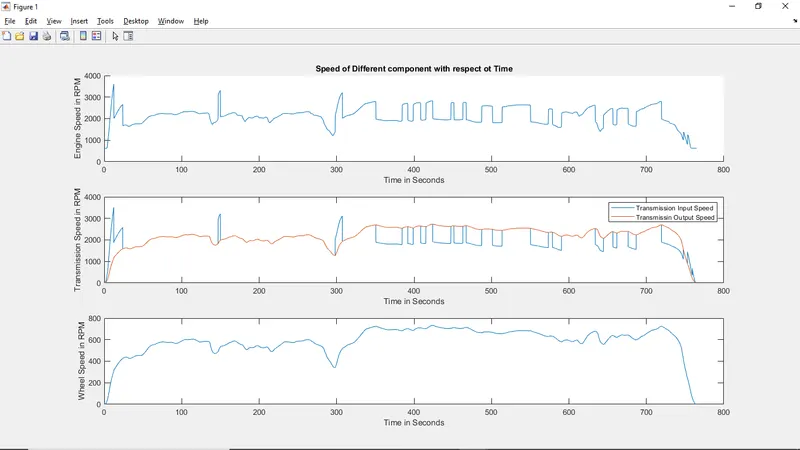
Figure 15: Speed of various component with respect to time for HWFET cycle.

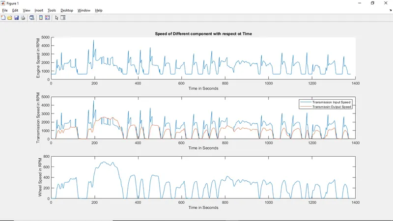
Figure 16: Speed for various component with respect to time for UDDS cycle.

4.3 Acclerator , Brake pedal pressed percentage, Gear command, Actual and Desired Speed and Total distance for HWFET and UDDS Drive Cycle

In HWFET cycle we can observe that brake pedal was less used as compared to the UDDS cycle because in HWFET cycle vehicle doesnot need the frequent start, stop. In UDDS cycle, the vehicle is mostly operated in second gear so the speed of transmission at input is always higher than the outspeed while In HWFET cycle, vehicle is mostly operated in fourth gear which is overdrive so we can see higher output speed of the transmission system. In HWFET cycle the vehicle travels a distance of around 16 km in around 800 seconds while In UDDS cycle vehicle travels a distance of around 12km in around 1400 seconds this implies, vehicle at HWFET cycle travels at higher velocity. The actual and desired speed for both cycle are similiar for both cycle. Figure 17 and 18 shows the acclerator , brake pedal pressed percentage, gear command , actual and desired speed and total distance for HWFET and UDDS cycle.

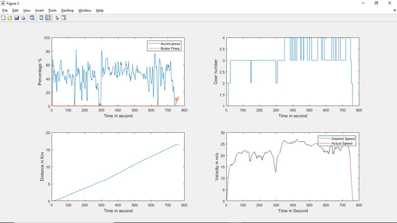
Figure 17: Acclerator, brake pedal pressed percentage,Gear command, distance and actual and desired speed of vehicle for HWFET cycle.

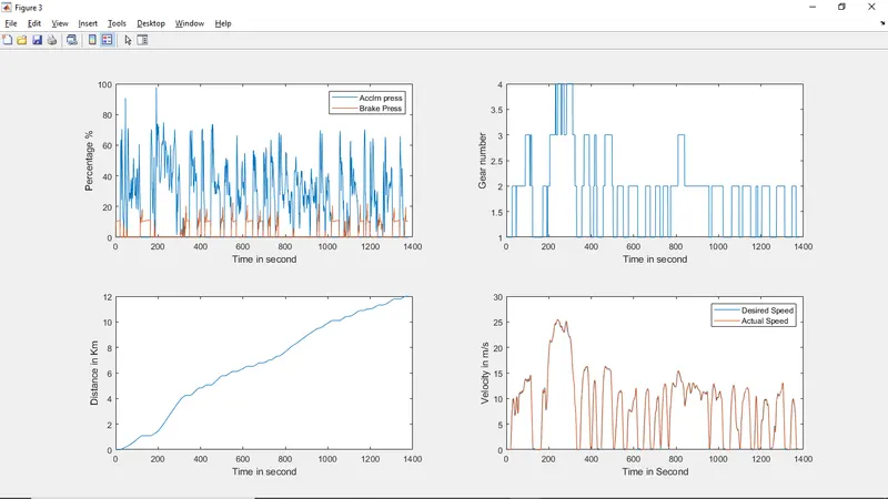
Figure 18:Acclerator, brake pedal pressed percentage,Gear command, distance and actual and desired speed of vehicle for UDDS cycle

4.4 Engine Torque ,Power , Fuel consumption rate and Total fuel consumed for HWFET and UDDS cycle

It was observed that, the maximum torque produce by the engine during UDDS cycle was around 150Nm for which the power of 48Kw was developed by engine at the fuel consumption of 4gm/sec. The total fuel consumed for the UDDS cycle was around 610gm. It was observed in the power plot that occurance of negative power was much higher which is due to the frequent brake request for UDDS cycle.For HWFET cycle, the maximum torque produced by the engine was around 120Nm for which the power of around 39Kw was developed by the engine at the fuel consumption of 3 gm/sec. The occurance of negative power was low as compared to the UDDS cycle as frequent braking was not required in highway. Figure 19 and 20 shows the Engine Torque, power, fuel consumption rate and total fuel consumed for the UDDS and HWFET cycle

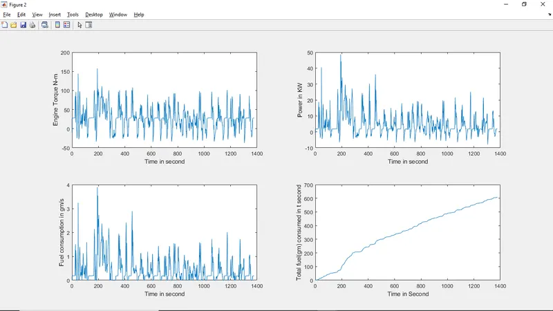
Figure 19:Engine Torque, power, fuel consumption rate and total fuel consumed for the UDDS cycle

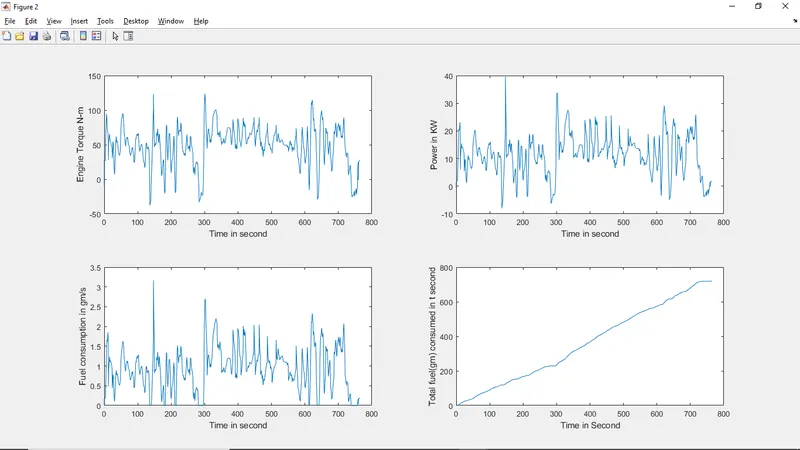
Figure 20: Engine Torque, power, fuel consumption rate and total fuel consumed for the HWFET cycle

4.5 Engine Operating Point for HWFET and UDDS Cycle

In HWFET cycle, most of the operating point lies sightly rightside of operating point which was their in the UDDS cycle. This means that for UDDS cycle most of the time the engine is operating at its lower efficiency point. Figure 21 and 22 shows the operating point for UDDS and HWFET cycle respectively.

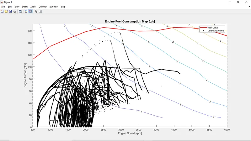
Figure 21: Engine Operating point for UDDS cycle

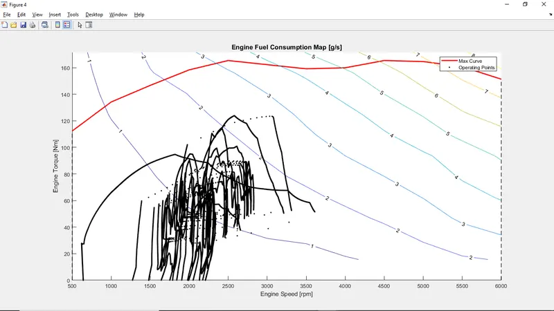
Figure 22: Engine operating point for HWFET cycle

4.6 Plot for Drive cycle

Figure 23 shows the HWFET drive cycle and 24 shows the UDDS drive cycle.

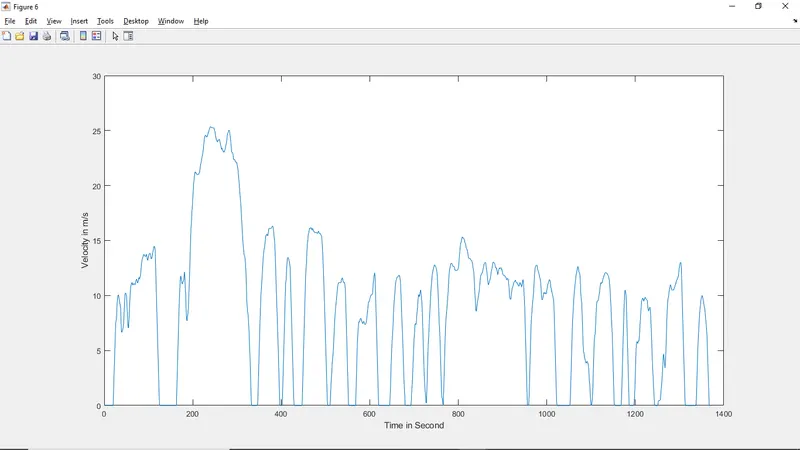
Figure 23: UDDS drive cycle

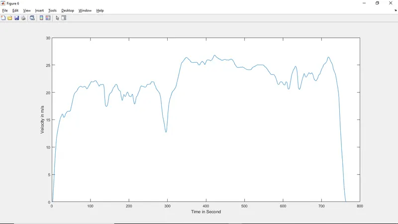
Figure 24: HWFET drive cycle

Conclusion:

It was seen that when the vehicle is subjected to frequent start and stop than the fuel consumed by the engine is high as seen in UDDS cycle while for HWFET cycle it was observed that the average power developed the engine was comparitavely higher than UDDS cycle.To overcome the energy loss during or to increase the milage of the vehicle hybrid vehicle seems best alternative as it stops the engine during idling as the features like regenerative braking can be effectively used to absorb some amount of power which is loss during braking of vehicle.

Reference:

1.G Mohan, F Assadian, S Longo,Comparative analysis of forward-facing models vs backwardfacing models in powertrain component sizing ,Department of Automotive Engineering, Cranfield University, United Kingdom .