Week 4.1 - Genetic Algorithm

Objectives:

• To optimise the stalagmite function.
• To find the global maxima of stalagmite function.

Theory:

 Stalagmite function is the basis representation of the stalagmite rock. This functions contains a various local maxima and a global maxima. Genetic algorithm is the search and optimization technic which imitates the process of natural evolution and can be used to find the value for maximum and minimum value of particular function. The different component of genetic algorithm are as follow:

• Fitness function
• Population of chromosome
• Selection according to fitness
• Crossover to produce new offspring
• Random mutation of new offspring.

Fitness function is the most pivotal part of the genetic algorithm and this is the function for which we are trying to get the optimum value. In our case ,stalagmite function is the fitness function. Chromosome of population are often bit string which mainly takes two value i.e. 0 and 1. Search process takes place by processing the chromosomes. These chromosome are assign to the fitness function and  based on the fitness function GA assign a score for it. During selection process, a fitter chromosome is selected to reproduce.During crossover, the sequence of chromosome are interchanged to produce new offspring.In mutation, bits of chromosome are randomly flipped. The working of genetic algorithms can be briefly explained in following steps:

1. In first step, population of chromosome is randomly generated.
2. With the help of fitness function f(x), calculate the fitness for each chromosome.
3. Repeat the following process untill the required number of offsprig have created

1. Select the pair of parent chromosome in such a way that, the same chromosome can be selected for more than one time as a parent chromosome.
2. With crossover proababilty, crossover the pair at randomly choosen point to form the two offspring.
3. If there is no crossover, than select two offspring  in such a way that they are the exact copy of their respective parent.
4. With mutation proability, mutate the two offspring and place the new chromosome as a new population

Use the new population as current population and repeat the process from step2.

Syntax for Genetic algorithm

 Based on the use of genetic algorithm the syntax of genetic algorithm can be as follow:

1. x=ga(fun,nvars)

where x is local unconstrained minimum, fun is the objective function and nvars is number of design variable of function , fun

2. x=ga(fun,nvars,A,b)

where A and b are linear inequality subjected to function ,fun.

3.x=ga(fun,nvars,A,b,Aeq,beq)

where Aeq and beq are linear equality subjected to function, fun.

4.x=ga(fun,navrs,A,b,Aeq,beq,lb,ub)

where, lb and ub are lower and upper bond of the variable x resp.

5.x=ga(fun,nvars,A,b,Aeq,beq,lb,ub,nonlcon)

6.x=ga(fun,navrs,A,b,Aeq,beq,lb,ub,nonlcon,options)

7.x=ga(fun,nvars,A,b,[],[],lb,ub,nonlcon,options,intcon)

8.x=ga(problem)

9.[x,fval]=ga(_)

10.[x,favl,exitflag,output]=ga(_)

11.[x,fval,exitflag,output,population,score]=ga(_)

Used of above syntax:

1. Synatax number 1 is used find local unconstrain minimum for x to the objective function (fun).
2. Syntax number 2 is used to local minimum x to function(fun),which is subjected to the linear inequality as A*x<=b.
3. Syntax number 3 is used to find local minimum for function which is subjected to linear equality in such a way that Aeq*x=beq and A*x<=b.
4. Syntax number 4 is used to find local minimum for the function fun for the range lb<=x<=ub.
5. In Synatax number 5 ,nonlcon is the function which take x and return vector C and Ceq which representsnon  linear inequalities  and equalities resp. ga minimizes the function in such a way that C(x)<=0 and Ceq(x)=0.
6. Syntax 6 is used when we need to change some optimization parameters.
7. Syntax 8 find the mimium for problem.
8. Syntax 9 , it returns the value for fitness function x as fval.
9. Syntax 10 , returns the reason for temination of ga as an interger exitflag and output contains the output form each generations as well as information regarding the performance of the algorithms.
10. Syntax 11 , returns matrix population whose rows are the final population and vectors scores of final population.

Coding logic:

Initally define the input. Now create the staglamite function and get the value of function for different inputs. Based on the requirement make some adjustement to get the maximum value from the function when ga search the solution. Now with the help of genetic algorithm get the maximum value. For more accurate result, use loops. When ga search beyond the workspace, confined the search area by using lower and upper bound. For getting much more accurate result, change some parameters by using optimoptions commands.

 Equation for stalagmite function:

 `f(x,y)=f1*f2*f3*f4`

`f_1=(sin(5.1pix+0.5))^6`

`f_2=exp(-4ln(2)*(x-0.0667)^2/0.64)`

`f_3=exp(-4ln(2)*(y-0.0667)^2/0.64)`

`f_4=(sin(5.1piy+0.5))^6`

Steps:

• Create an input variables.
• Convert 1D array to 2d array.
• Define a function name stalagmite.
• By using nested loop, provide the input value for stalagmite function.
• Create the surface plot with the help of input variables and function result.
• Make necessary adjustment to find the maximum value for the given fitness function.
• With the help of genetic algorithm , find the maximum value for the function.
• Use the genetic algorithm inside for loop(for more iteration) to get more accurate result.
• To improve the accuracy result for maximum value, use upper and lower bound or increase the size of population. By doing this accuracy of the result will increase.
• By using subplot and plot command , plot the result for bounded, unbounded and Increasing result.
• Use marker to visualize the maximum point search by ga for 3D plot.

Codes:

a. Codes for stalagmite Function

function f=stalgmite(input)
x=input(1);
y=input(2);
f1= (sin(5.1*pi*x+0.5))^6;
f2=(sin(5.1*pi*y+0.5))^6;
f3=exp(-4*log(2)*(((x-0.0667)^2))/0.64);
f4=exp(-4*log(2)*(((y-0.0667)^2))/0.64);
f=-1*(f1*f2*f3*f4);  %-ve sign is used to convert minimum value to maximum value
end

 b.Codes which is common for all cases:

clear all
close all
clc

x=linspace(0,0.8,150); %creating the input parameter
y=linspace(0,0.8,150);

[xx,yy]=meshgrid(x,y); %converting 1D array to 2D array
n=100;  %Number of iteration
for i=1:length(xx)
    for j=1:length(yy)
        input(1)=xx(i,j);
        input(2)=yy(i,j);
        f(i,j)=stalgmite(input); %getting the value for stalagmite function by callling the function
    end
end

c.Codes for Unbound Conditions:

clear all
close all
clc

x=linspace(0,0.8,150); %creating the input parameter
y=linspace(0,0.8,150);

[xx,yy]=meshgrid(x,y); %converting 1D array to 2D array
n=100;  %Number of iteration
for i=1:length(xx)
    for j=1:length(yy)
        input(1)=xx(i,j);
        input(2)=yy(i,j);
        f(i,j)=stalgmite(input); %getting the value for stalagmite function by callling the function
    end
end



%case1 For Unbound condition
tic
for i= 1:n
    [x,fval(i)]=ga(@stalgmite,2); %getting maximum value using ga
    
    xopt1(i)=x(1); %creating the new variable for plotting purpose
    yopt1(i)=x(2); %creating the new variable for plotting purpose
end

time1=toc;   %It will show time for completion of Unbound condition


%plotting
%case1 Unbound condition

figure(1)

subplot(2,1,1)
surf(xx,yy,-f);
title('Unbound Condition')
shading interp
hold on


%Plotting the value which ga gets
plot3(xopt1,yopt1,-fval,'marker','o','markersize',5,'markerfacecolor','r');
xlabel('X axis');
ylabel('y axis');

subplot(2,1,2)
plot(-fval)
xlabel('Iteration');
ylabel('maximum value')
hold off

Output for time:
time1 =

    7.9211

d.Codes For Bound Conditions:

clear all
close all
clc

x=linspace(0,0.8,150); %creating the input parameter
y=linspace(0,0.8,150);

[xx,yy]=meshgrid(x,y); %converting 1D array to 2D array
n=100;  %Number of iteration
for i=1:length(xx)
    for j=1:length(yy)
        input(1)=xx(i,j);
        input(2)=yy(i,j);
        f(i,j)=stalgmite(input); %getting the value for stalagmite function by callling the function
    end
end


%case2 Bounded Condition
tic
for i= 1:n
    [x,fval1(i)]=ga(@stalgmite,2,[],[],[],[],[0;0],[0.8;0.8]); %[00] and [0.8 0.8 are the boundary for given function
    xopt2(i)=x(1);
    yopt2(i)=x(2);
end
time2=toc;  %It will show time for completion of Bound condition

%case 2 bound condition

figure(2)

subplot(2,1,1)
surf(xx,yy,-f);
title('Bound Condition')
shading interp

hold on
plot3(xopt2,yopt2,-fval1,'marker','o','markersize',5,'markerfacecolor','r');
xlabel('X axis');
ylabel('y axis');

subplot(2,1,2)
plot(-fval1)
xlabel('Iteration');
ylabel('maximum value')
hold off

Output for time2:
time2 =

    8.8596

e.Codes for Increasing Population case:

clear all
close all
clc

x=linspace(0,0.8,150); %creating the input parameter
y=linspace(0,0.8,150);

[xx,yy]=meshgrid(x,y); %converting 1D array to 2D array
n=100;  %Number of iteration
for i=1:length(xx)
    for j=1:length(yy)
        input(1)=xx(i,j);
        input(2)=yy(i,j);
        f(i,j)=stalgmite(input); %getting the value for stalagmite function by callling the function
    end
end

%case3: Increasing popuation
tic
options=optimoptions('ga','populationsize',1000); %To change default value of 50 to 1000
for i= 1:n
    [x,fval2(i)]=ga(@stalgmite,2,[],[],[],[],[0;0],[0.8;0.8],[],[],options);
    xopt3(i)=x(1);
    yopt3(i)=x(2);
end
time3=toc;


%case3 population increasing

figure(3)

subplot(2,1,1)
surf(xx,yy,-f);
title('Increasing population')
shading interp
hold on

plot3(xopt3,yopt3,-fval2,'marker','o','markersize',5,'markerfacecolor','r');
xlabel('X axis');
ylabel('y axis');

subplot(2,1,2)
plot(-fval2)
xlabel('Iteration');
ylabel('maximum value');
hold off

Output for time3:
time3 =

  115.4487

f. Whole Codes :

clear all
close all
clc

x=linspace(0,0.8,150); %creating the input parameter
y=linspace(0,0.8,150);

[xx,yy]=meshgrid(x,y); %converting 1D array to 2D array
n=100;  %Number of iteration
for i=1:length(xx)
    for j=1:length(yy)
        input(1)=xx(i,j);
        input(2)=yy(i,j);
        f(i,j)=stalgmite(input); %getting the value for stalagmite function by callling the function
    end
end



%case1 For Unbound condition
tic
for i= 1:n
    [x,fval(i)]=ga(@stalgmite,2); %getting maximum value using ga
    
    xopt1(i)=x(1); %creating the new variable for plotting purpose
    yopt1(i)=x(2); %creating the new variable for plotting purpose
end

time1=toc;   %It will show time for completion of Unbound condition


%case2 Bounded Condition
tic
for i= 1:n
    [x,fval1(i)]=ga(@stalgmite,2,[],[],[],[],[0;0],[0.8;0.8]); %[00] and [0.8 0.8 are the boundary for given function
    xopt2(i)=x(1);
    yopt2(i)=x(2);
end
time2=toc;  %It will show time for completion of Bound condition

%case3: Increasing popuation
tic
options=optimoptions('ga','populationsize',1000); %To change default value of 50 to 1000
for i= 1:n
    [x,fval2(i)]=ga(@stalgmite,2,[],[],[],[],[0;0],[0.8;0.8],[],[],options);
    xopt3(i)=x(1);
    yopt3(i)=x(2);
end
time3=toc;

time=[time1 time2 time3];
%plotting
%case1 Unbound condition

figure(1)

subplot(2,1,1)
surf(xx,yy,-f);
title('Unbound Condition')
shading interp
hold on


%Plotting the value which ga gets
plot3(xopt1,yopt1,-fval,'marker','o','markersize',5,'markerfacecolor','r');
xlabel('X axis');
ylabel('y axis');

subplot(2,1,2)
plot(-fval)
xlabel('Iteration');
ylabel('maximum value')
hold off

%case 2 bound condition

figure(2)

subplot(2,1,1)
surf(xx,yy,-f);
title('Bound Condition')
shading interp

hold on
plot3(xopt2,yopt2,-fval1,'marker','o','markersize',5,'markerfacecolor','r');
xlabel('X axis');
ylabel('y axis');

subplot(2,1,2)
plot(-fval1)
xlabel('Iteration');
ylabel('maximum value')
hold off


%case3 population increasing

figure(3)

subplot(2,1,1)
surf(xx,yy,-f);
title('Increasing population')
shading interp
hold on

plot3(xopt3,yopt3,-fval2,'marker','o','markersize',5,'markerfacecolor','r');
xlabel('X axis');
ylabel('y axis');

subplot(2,1,2)
plot(-fval2)
xlabel('Iteration');
ylabel('maximum value');
hold off

%visua;ization for study time
figure(4)
bar(time)
title('value of time for different condition');

Result:

a.For Unbound Conditions:

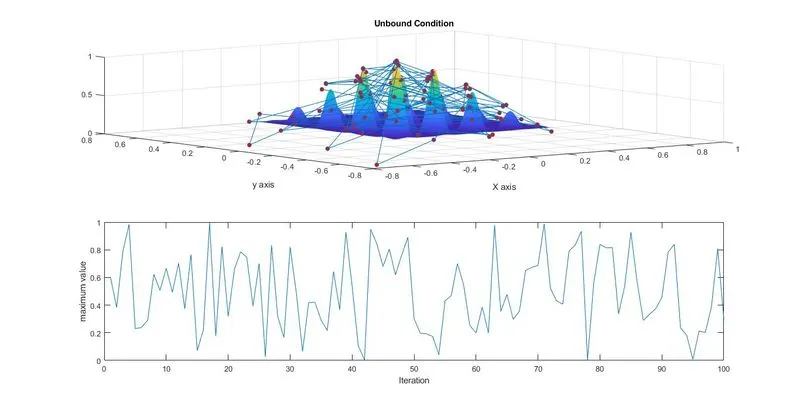
From above figure. it was clear that when the boundary is not specified than ga not only search with the workspace but also tries to move out of the workspace. In second plot we can also observe that ga gets us a maximum value for the function 4 times which is between 0-10 iteration,10-20 iteration,60-70iteration and 70-80 iteration as observed in above figure.It was also observed that, the value ga gets is in the range of 0-1 and the accuracy is also low.

b.For Bound Conditions:

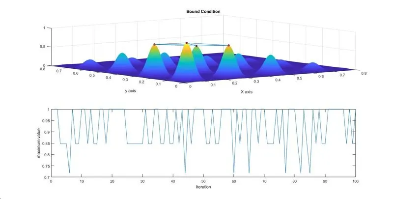
From above figure it is clear that when we provide boundary to the ga it often goes to the local maxima and global maxima point. In second plot we can also observe that the range of value which ga gets also reduces form 0-1 to 0.7 to 1.And Ga finds global maxima for much time when compared with unbound conditions.

c.Increasing Population:

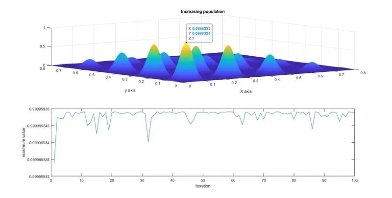
From above figure it is clear that ga tends to find global maxima when number of population is increased. Further it was also observed that the range at which ga search also reduces as compared with bound and uncound condition. The range was reduced from 0.7 to 1 to 0.9999983 to 1 as indicatedin figure. and the maximum value of stalagmite function was found to be 1 at x 0.066335 and y at 0.0668334.

d.Time for simulation for different cases:

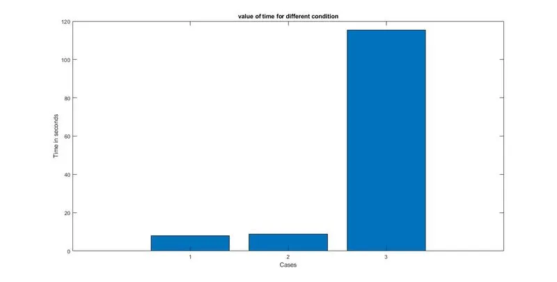
Case1: For unbound Conditions

Case2: For Bound Conditions

Case3: For Increasing Population

Conclusion:

Stalagmite function has been optimized and the maximum value of the function was found to be 1. It was observed that with increase in population of the chromosome , time taken to simulate the result will be more.

References:

1. https://www.whitman.edu/Documents/Academics/Mathematics/2014/carrjk.pdf, last accessed Sept 2,2021.
2. https://www.iitg.ac.in/rkbc/CE602/CE602/Genetic%20Algorithms.pdf last accessed, Sept2,2021
3. https://www.egr.msu.edu/~goodman/GECSummitIntroToGA_Tutorial-goodman.pdf last accessed, Sept2,2021
4. http://www.cs.cmu.edu/~02317/slides/lec_8.pdf, last accessed Sept2 2021
5. https://in.mathworks.com/help/gads/ga.html last accessed Sept 3,2021