Project 1
Aim
To develop a forward energy-based fuel consumption model of a conventional vehicle.
Objectives
To compute the fuel economy numbers for the given vehicle (kmpl) on the urban cycle (UDDS) and highway cycle (HWFET).
Analyze the Vehicle operating points at different drive cycles .
To Plot the engine operating points on the engine fuel map.
To Plot the time trace for engine, transmission input, transmission output and wheel speed on one plot.
Forward Model of a Conventional Vehicle System
A forward model of a conventional vehicle system is a computer simulation that predicts the vehicle's behavior in response to driver inputs and environmental conditions. The model is typically composed of the following components:
- Driver model: This model simulates the driver's behavior, such as acceleration, braking, and steering.
- Vehicle dynamics model: This model simulates the vehicle's physical dynamics, such as its mass, inertia, and aerodynamics.
- Powertrain model: This model simulates the vehicle's powertrain, including the engine, transmission, and differential.
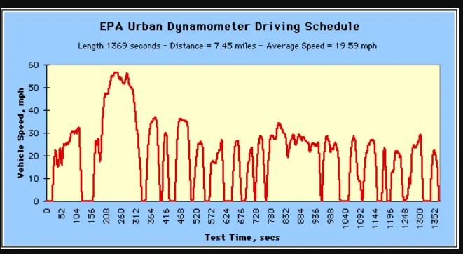
Urban Dynamometer Driving Schedule (UDDS)
The EPA Urban Dynamometer Driving Schedule (UDDS) is commonly called the "LA4" or "the city test" and represents city driving conditions. It is used for light duty vehicle testing. The UN/ECE Regulation 53 refers to the EPA UDDS as the "Test Equivalent to the Type 1 Test (verifying emissions after a cold start).
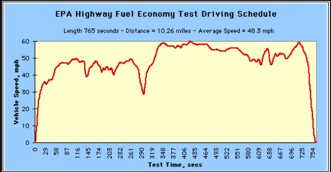
Highway Fuel Economy Driving Schedule (HWFET)
Represents highway driving conditions under 60 mph.
Intial Matlab code
Initialization file for loading the variables for the Conventional vehicle simulation model .
%% Vehicle Parameters
M = 1500;       % Vehicle weight [kg]
Cr = 0.015;     % Rolling resistance coefficient
Rw = 0.35;      % Rolling radius [m]
Cd = 0.33;      % Drag coefficient
Af = 2;         % Frontal area [m2]
rhoa = 1.225;   % Air density [kg/m3]
Vwind = 0;      % Wind velocity [kmph]
g = 9.81;       % Gravitational acceleration [m/s2]
theta = 0;      % Slope [deg]
myu_road_tire = 1; % Coefficient of friction between tire - road interface

%% Powertrain Parameters
FDR = 3.73;                         % Final Drive Ratio / Diff Ratio
DiffEff = 0.99;                     % Differential efficiency (assumed independent of operating conditions)

NumGear = 4;                        % Number of gears in transmission
TransGear = 1:NumGear;            % Transmission Gears
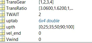
TransRatio = [3.06, 1.62, 1, 0.7];  % Corresponding Transmission ratios
TransEff = 0.90;                    % Transmission efficiency (assumed independent of operating conditions)

TC_SR = [0, .5, .6, .7, .8, .87, .92, .94, .96, .97, 1];   % Torque Converter Speed Ratio (Matlab default) -> TurbSpd/PumpSpd
TC_TR = [2.232, 1.5462, 1.4058, 1.2746, 1.1528, 1.0732, 1.0192, 1, 1, 1, 1];   % Torque Converter Torque Ratio (Matlab default) -> TurbTrq/PumpTrq
TC_Cf = 1e-4 * [.72558, .66322, .63463, .59042, .51331, .4144, .29287, .22444, .12186, .04386, 0]; % Torque Converter Capacity Factor (Matlab default) -> PumpTrq/PumpSpd^2 [Nm/rpm^2]

load Vehicle_Data/Engine_data_1_9L_Saturn_95kW
load Vehicle_Data/Trans_Shift_map

%% Driver Parameters
Kp = 10;                    % P gain for driver PI model
Ki = 1;                     % I gain for driver PI model
Drive_Cycle_Select = 1;     % Drive cycle selection

% Drive cycle values in m/s

if Drive_Cycle_Select == 1
    load DriveCycles/UDDS;

elseif Drive_Cycle_Select == 2
    load DriveCycles/HWFET;

elseif Drive_Cycle_Select == 3
    load DriveCycles/FTP;

elseif Drive_Cycle_Select == 4
    load DriveCycles/US06;

elseif Drive_Cycle_Select == 5
    load DriveCycles/NEDC;

elseif Drive_Cycle_Select == 6
    load DriveCycles/WLTP;

end

time_end = cyc_time(end);
vel_end = cyc_vel(end);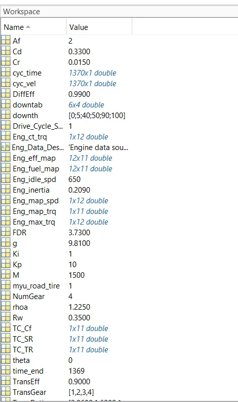
Simulink model
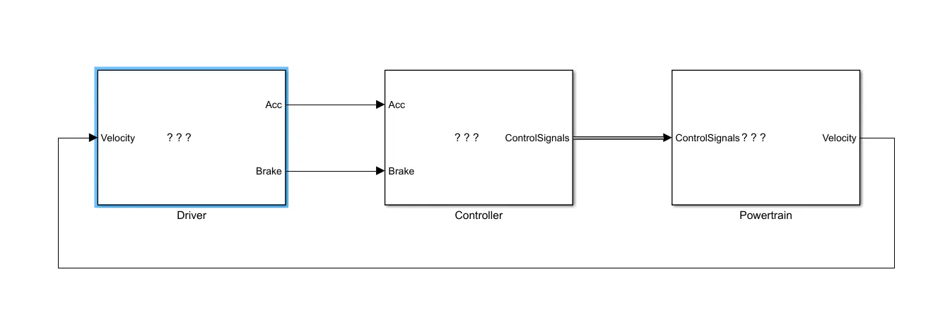
The Vehicle model of conventional vehicle system consists of three major blocks
Driver block
Controller block
Powertrain block
Driver block
It is basic PI controller that generates accelerator and brake pedal outputs to match the desired
and actual vehicle speeds.
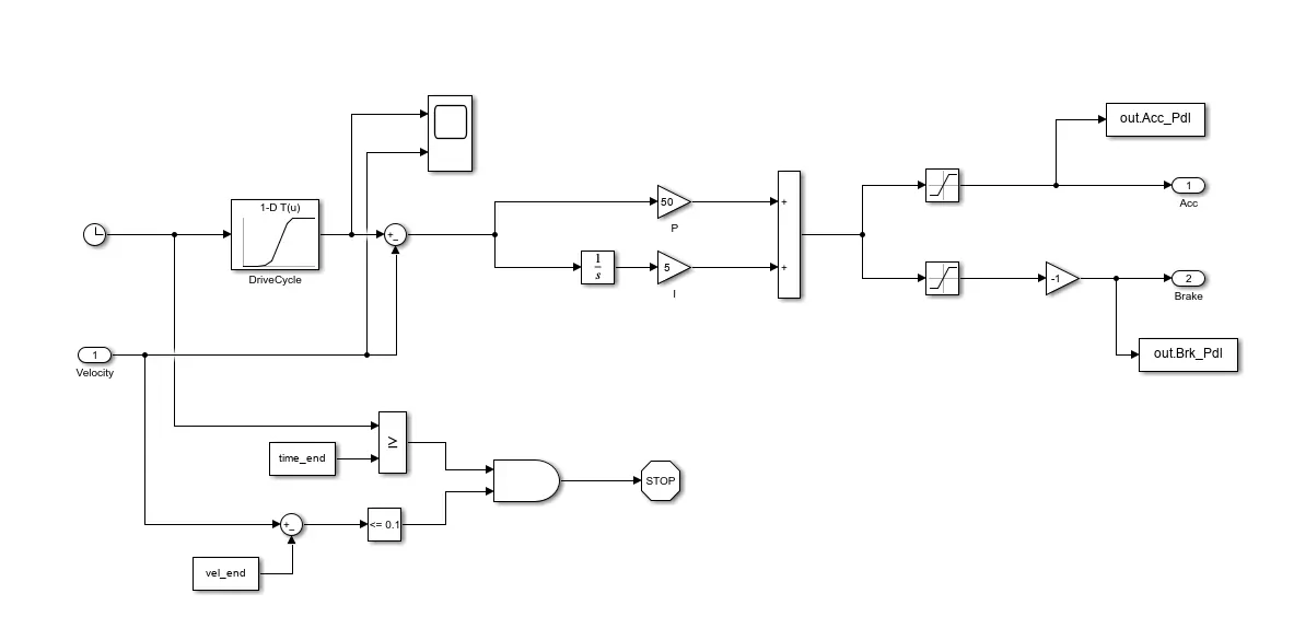
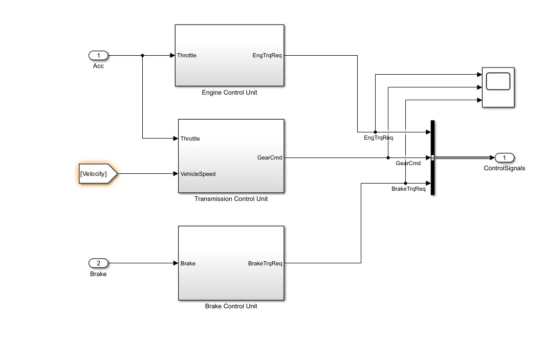
Controller model
It is the brains of the vehicle, representing the electronic controls units. Based on the driver inputs, it generates desired engine torque, desired transmission gear and desired brake torque.
Engine control unit
This component simulates the behavior of the engine and predicts its torque output.
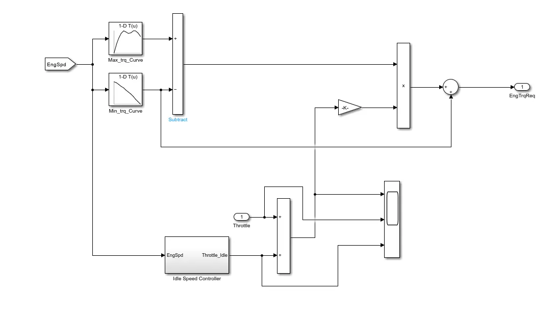
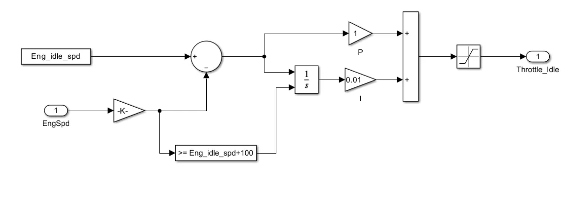
Idle Speed Controller
It monitors and controls engine idle speed and thus maintaining constant speed improves fuel economy.
Brake Control unit
It monitors and controls the braking system. It receives input signals from various brake system sensors, such as the wheel speed sensors, brake pressure sensor, and brake pedal sensor. It then uses this information to calculate the desired braking force and send signals to the brake actuators to apply the brakes. 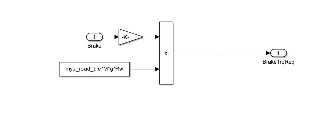
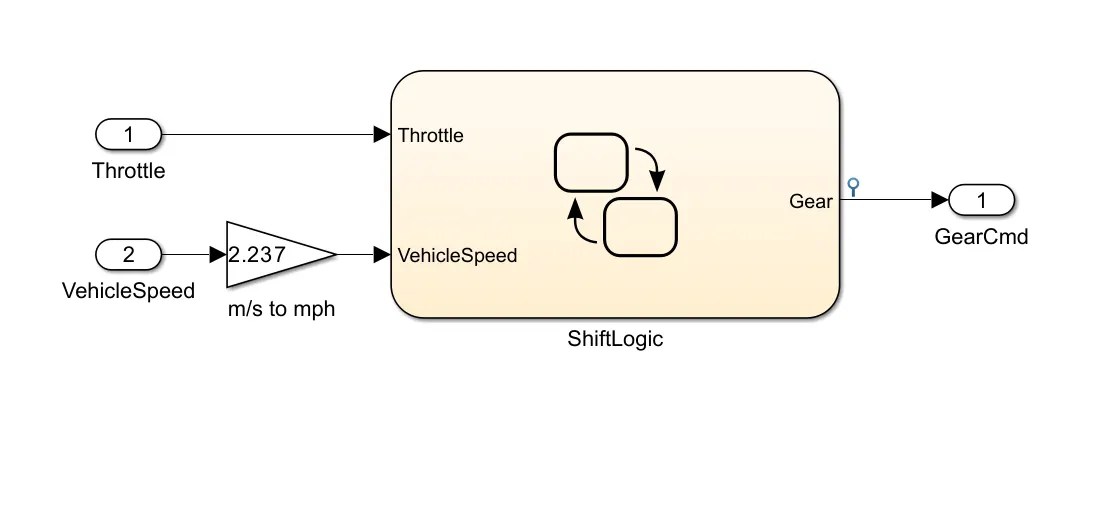
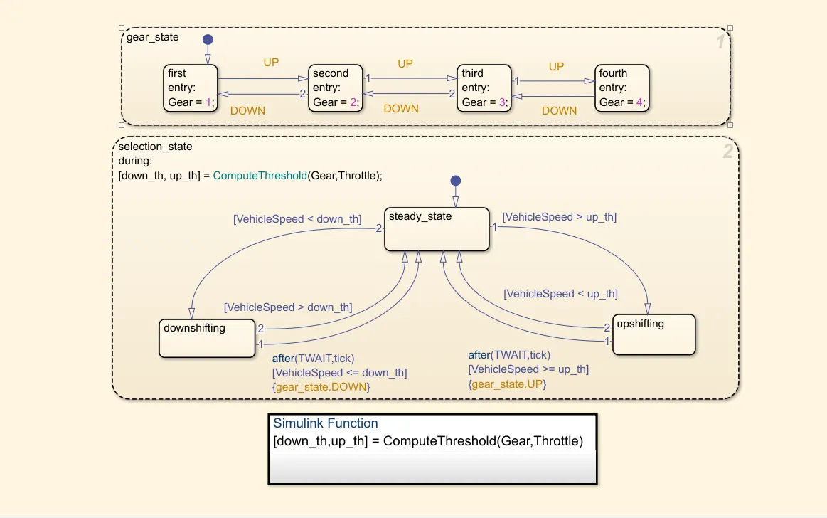
Transmission control unit
This component simulates the behavior of the transmission and predicts its gear ratio and output torque.
Power Train Model
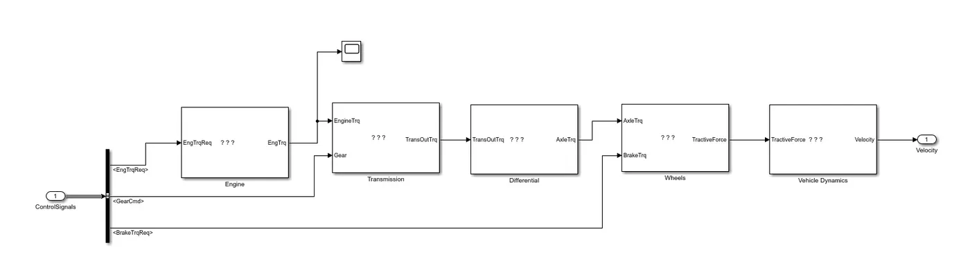
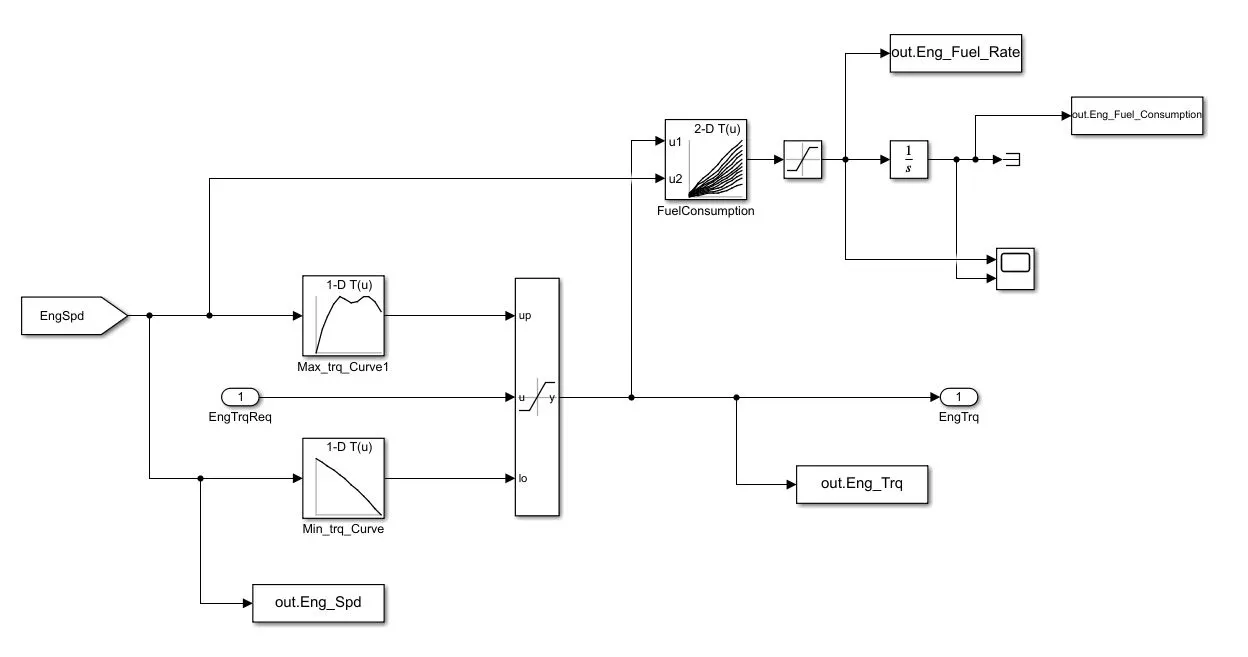
The engine model simulates the behavior of the engine and predicts its torque output. It takes into account the engine's characteristics, such as its displacement, number of cylinders, and combustion cycle.
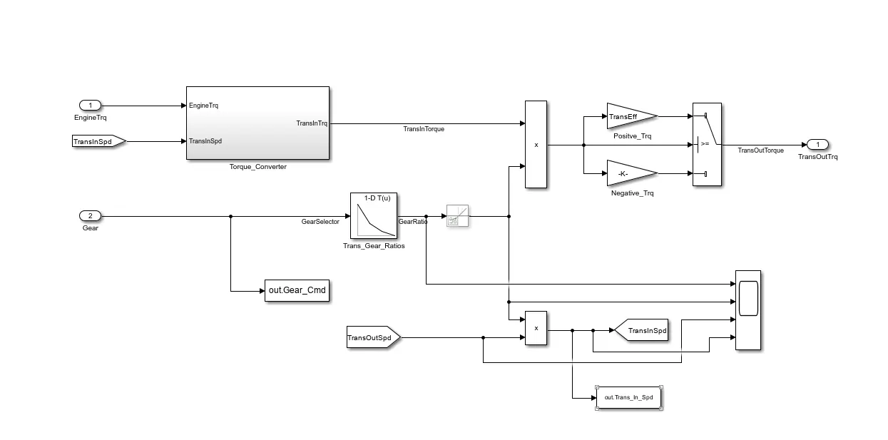
The transmission model simulates the behavior of the transmission and predicts its gear ratio and output torque. It takes into account the transmission's characteristics, such as its number of gears, gear ratios, and torque converter efficiency.
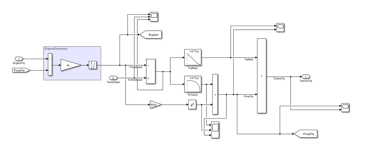
A torque converter in a conventional vehicle is a fluid coupling that transfers rotating power from the engine to the transmission. It is located between the engine's flexplate and the transmission's input shaft.
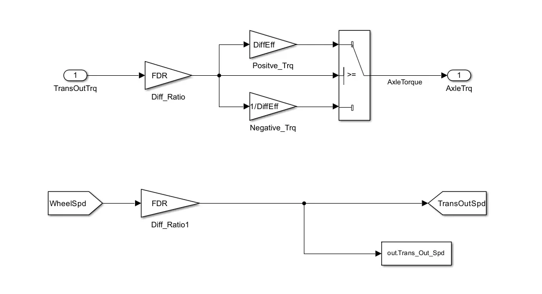
Differentials
A differential in a conventional vehicle is a device that allows the two wheels on an axle to rotate at different speeds. This is necessary when the vehicle is turning a corner, as the outer wheel needs to travel further than the inner wheel.
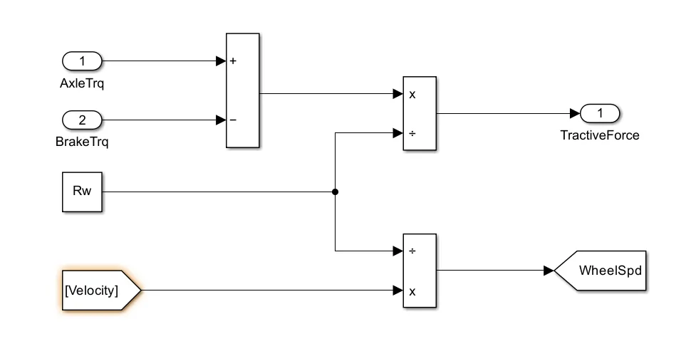
Wheels
They are responsible for transmitting power from the engine to the road. Wheels also play an important role in the vehicle's suspension and braking systems.
Vehicle Dyamics Block
The vehicle dynamics model simulates the dynamics of the vehicle, including the forces and torques that act on it. It takes into account the vehicle's characteristics, such as its mass, aerodynamic drag, and rolling resistance.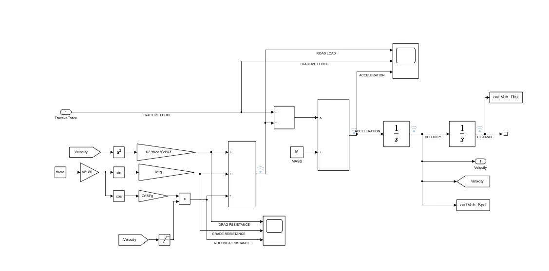
%% Postprocessing File

Time = out.tout;
Acc_Pdl = out.Acc_Pdl;          % Accelerator pedal [%]
Brk_Pdl = out.Brk_Pdl;          % Brake pedal [%]
Gear_Cmd = out.Gear_Cmd;        % Transmission gear
Trans_In_Spd = out.Trans_In_Spd*30/pi;  % Transmission input speed [rpm]
Trans_Out_Spd = out.Trans_Out_Spd*30/pi;% Transmission output speed [rpm]
Eng_Trq = out.Eng_Trq;          % Engine brake torque [Nm]
Eng_Spd = out.Eng_Spd*30/pi;    % Engine speed [rpm]
Eng_Fuel_Consump = out.Eng_Fuel_Consumption;    % Engine fuel consumption [g]
Veh_Dist = out.Veh_Dist/1000;   % Distance traveled by vehicle [km]
Veh_Spd = out.Veh_Spd*18/5;     % Vehicle speed [kmph]
WheelSpd=out.WheelSpd;            % wheel speed [rpm]
Eng_Fuel_rate=out.Eng_Fuel_Rate;

%% Data Analysis
Eng_Pwr = Eng_Spd.*pi./30.*Eng_Trq./1000;   % Engine brake power [kW]
rho_petrol = 0.7197;                    % Density of petrol [kg/L]
kmpl = Veh_Dist(end)/(Eng_Fuel_Consump(end)/1000/rho_petrol);    % Fuel economy [kmpl]

%Display Fuel Economy of the Cycle
fprintf('nFuel Economy = %2.2fkmplnn',kmpl);


%% Plotting vehicle characteristics time trace to Engine speed, Engine Torque, Engine Power, And Engine fuel rate, Engine fuel consumption
%% Plotting engine operating points on engine fuel map

figure(1)
hold on; grid on;
plot(Time,Trans_In_Spd, 'linewidth', 1, 'Color', 'black')
plot(Time,Trans_Out_Spd, 'linewidth', 1, 'Color', 'red')
plot(Time,WheelSpd, 'linewidth', 1, 'Color', 'green')
xlabel('time [s]'); ylabel('speed [rpm]');
xlim([0, Time(end)]); ylim([0, 6000]); legend('Trans In Spd','Trans Out Spd','WheelSpd');
%% Plotting torque ,power,fuel rate,fuel consumption

figure(2)

subplot(4,1,1)
grid on;
plot(Time, Eng_Trq, 'linewidth', 1, 'Color', 'black');
xlabel('time [s]'); ylabel('engine torque [Nm]');
xlim([0, Time(end)]);

subplot(4,1,2)
grid on;
plot(Time, Eng_Pwr, 'linewidth', 1, 'Color', 'blue');
xlabel('time [s]'); ylabel('engine power [Nm]');
xlim([0, Time(end)]);

subplot(4,1,3)
grid on;
plot(Time,Eng_Fuel_rate, 'linewidth', 1, 'Color', 'green');
xlim([0, Time(end)]);
xlabel('Time [s]'); ylabel('engine fuel rate');

subplot(4,1,4)
grid on;
plot(Time,Eng_Fuel_Consump, 'linewidth', 1, 'Color', 'red');
xlim([0, Time(end)]);
xlabel('Time [s]'); ylabel('engine fuel consumption');
%% Plotting vehicle characteristics time trace
figure(3)
subplot(4,1,1)
hold on; grid on;
plot(Time, Acc_Pdl, 'linewidth', 1, 'Color', 'black');
plot(Time, Brk_Pdl, 'linewidth', 1, 'Color', 'red'); ylabel('Pedal [%]');
xlim([0, Time(end)]);
legend('Accel','Brake');

subplot(4,1,2)
hold on; grid on;
plot(Time, Gear_Cmd, 'linewidth', 1, 'Color', 'black');
xlim([0, Time(end)]);
xlabel('Time [s]'); ylabel('Gear');

subplot(4,1,3)
hold on; grid on;
plot(cyc_time,(cyc_vel.*(18./5)), 'linewidth', 1, 'Color', 'black');
plot(Time, Veh_Spd, 'linewidth', 1, 'Color', 'red');
ylabel('velocity'); xlabel('Time [s]');
xlim([0, Time(end)]);
legend('desired speed','Actual speed');

subplot(4,1,4)
hold on; grid on;
plot(Time, Veh_Dist, 'linewidth', 1, 'Color', 'black');
xlim([0, Time(end)]);
xlabel('Time [s]'); ylabel('distance [km]');

%% Plotting engine operating points on engine fuel map

figure('Name','Engine Operating Points');
hold on; grid on;
title('Engine Operating Points','fontsize',12);
p1=plot(Eng_map_spd*30/pi,Eng_max_trq,'linewidth',2,'color','r');
p2=line([Eng_map_spd(end)*30/pi Eng_map_spd(end)*30/pi],[0 Eng_max_trq(end)]);
set(p2,'linewidth',1,'linestyle','--','color','k');
p3=line([Eng_map_spd(1)*30/pi Eng_map_spd(1)*30/pi],[0 Eng_max_trq(1)]);
set(p3,'linewidth',1,'linestyle','--','color','k');
[c,h] = contour(Eng_map_spd'*30/pi,Eng_map_trq,Eng_fuel_map');
clabel(c,h);
xlabel('Engine Speed [rpm]'); ylabel('Engine Torque [Nm]');
title('Engine Fuel Consumption Map [g/s]');
p4 = plot(Eng_Spd,Eng_Trq,'.','color','k');
legend([p1 p4],{'Max Curve','Operating Points'});
axis([Eng_map_spd(1)*30/pi Eng_map_spd(end)*30/pi 0 Eng_map_trq(end)]);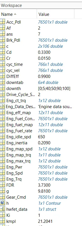
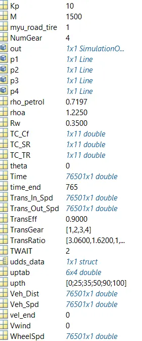
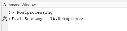
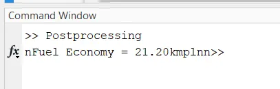
Fuel economy numbers (kmpl) for HWFET cycle = 21.20 Kmpl
UDDS Cycle
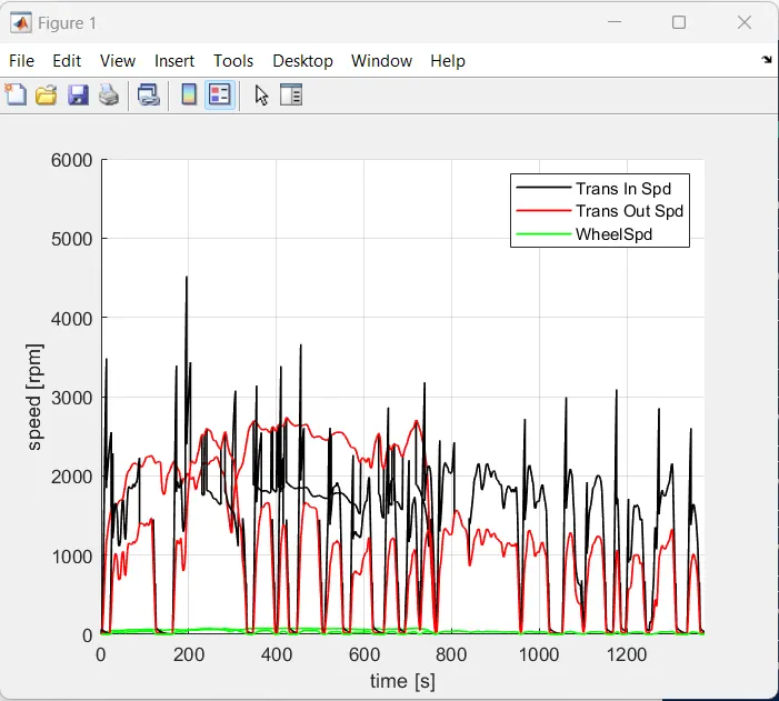
Plots for engine , transmission input , transmission output , and wheel speed
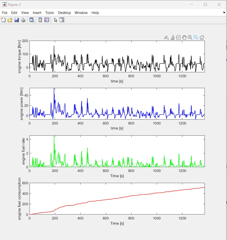
Plot engine torque, engine power, fuel rate and fuel consumption.
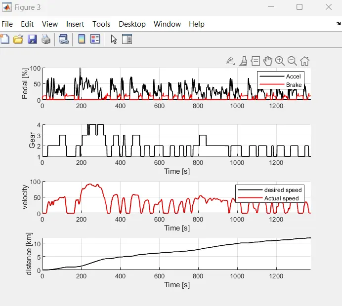
Plot accelerator and brake pedal, gear command, vehicle desired and actual speed, vehicle distance
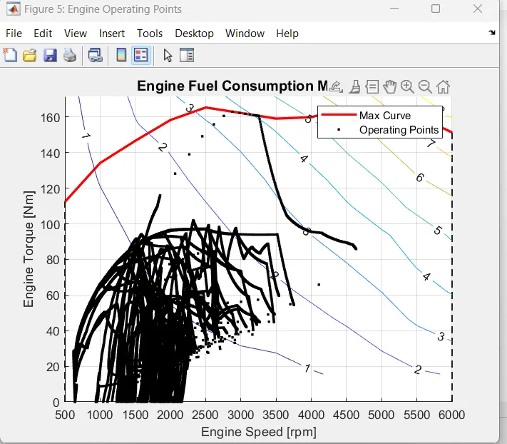
Plots for engine operating points on engine fuel map
Drive Cycle and Actual Velocity in UDDS Cycle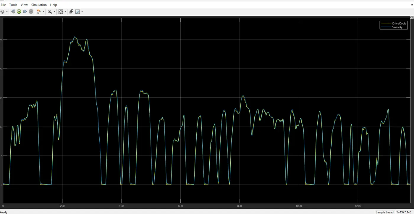
Engine Fuel flow and Fuel consumption in UDDS Cycle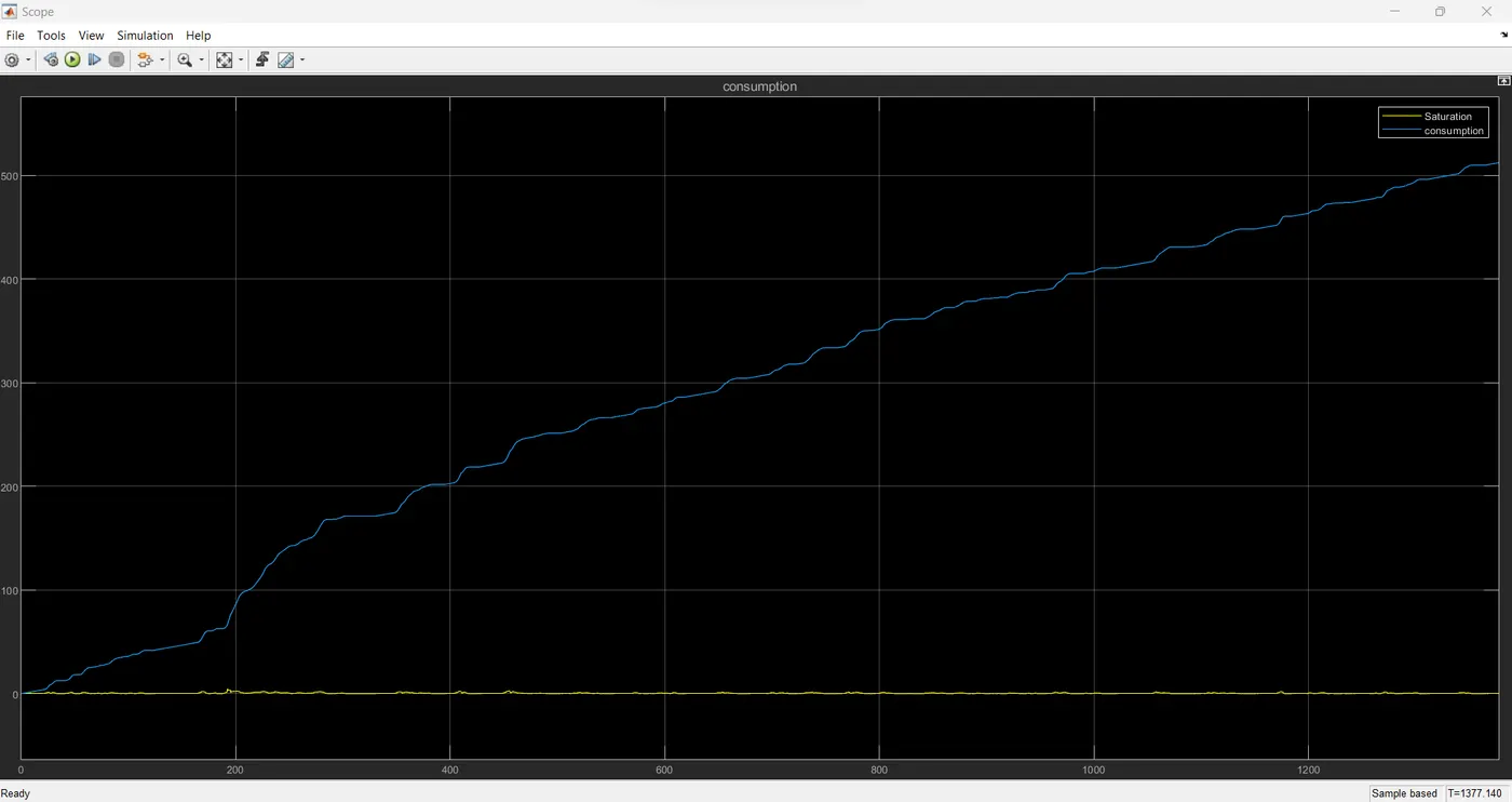
Engine Torque output in UDDS Cycle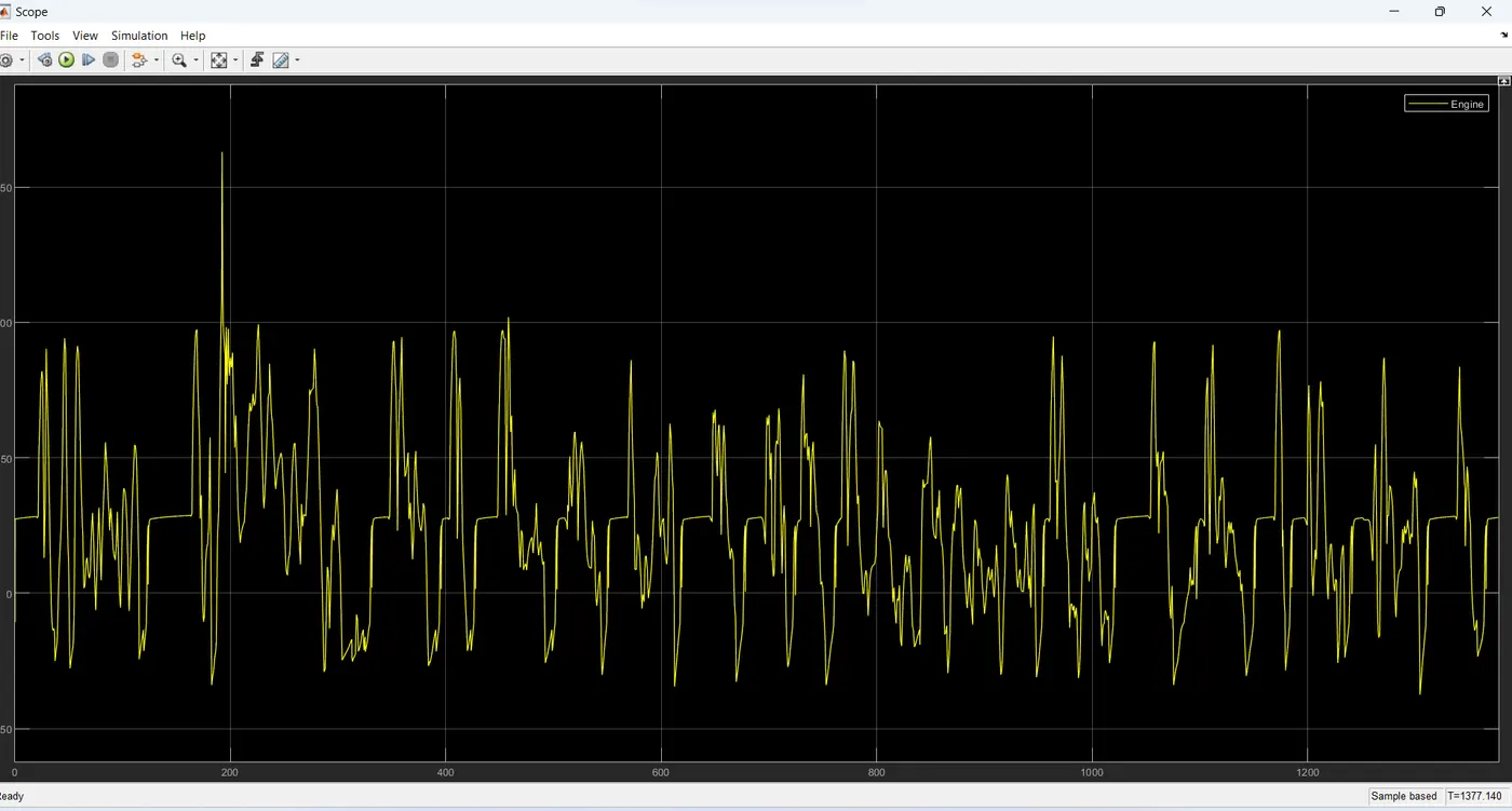
Engine Torque , Brake Torque in UDDS Cycle
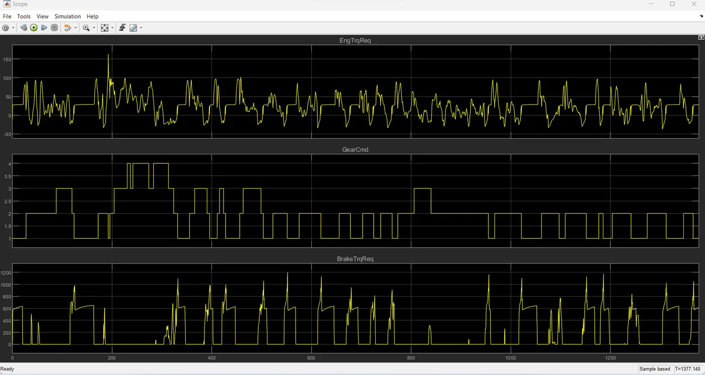
Gear Ratio , Transmission input , Transmission output in UDDS Cycle.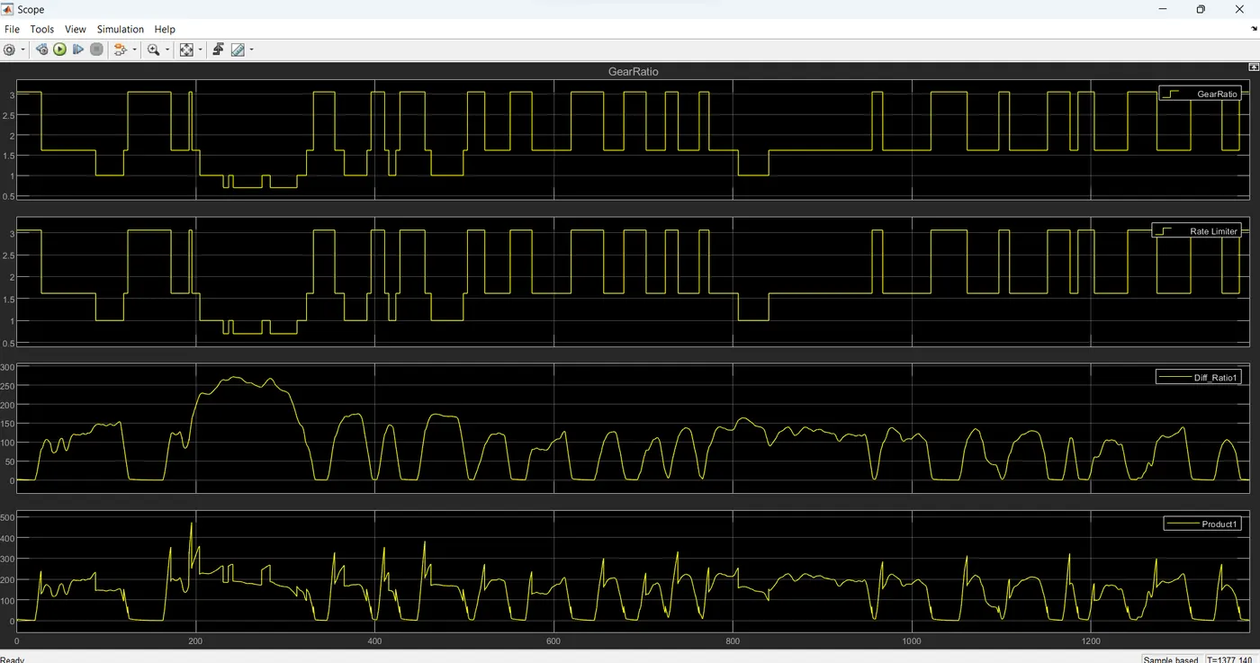
Pump speed , Turbine speed in UDDS Cycle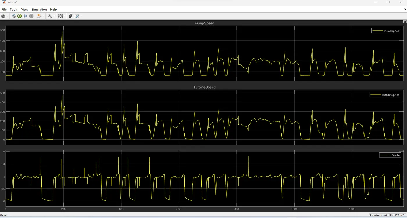
Road load , Tractive force and Accelaration in UDDS Cycle
Drag resistance and Rolling resistance in UDDS Cycle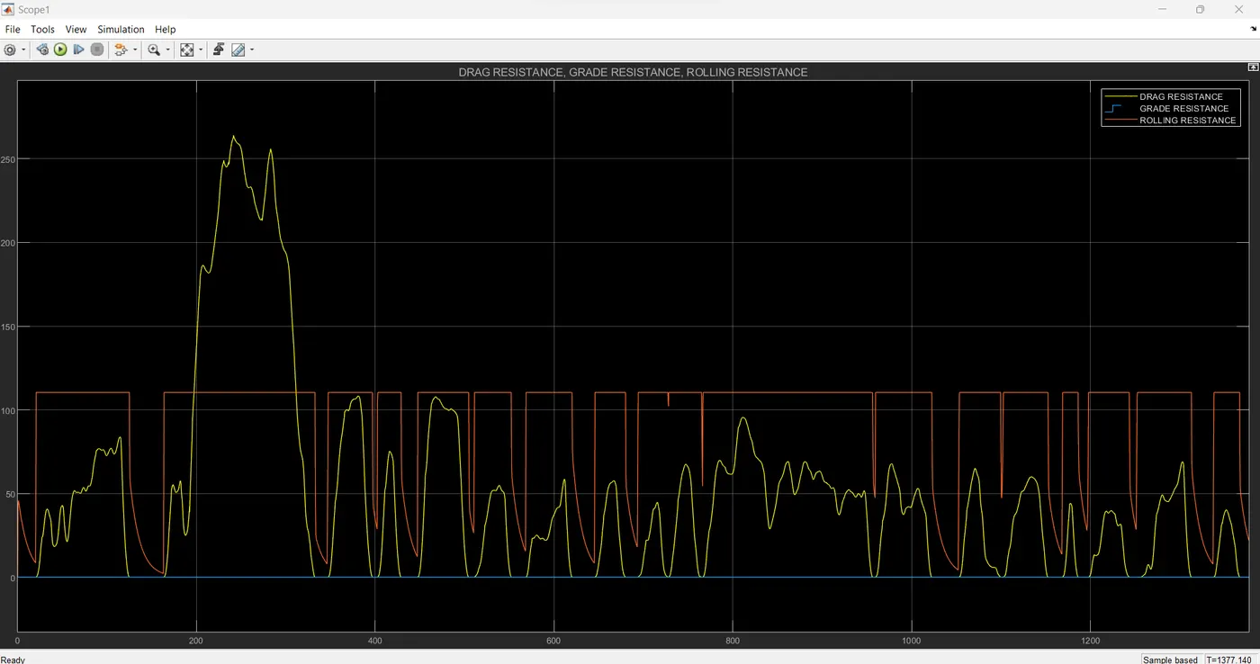
Torque ratio and Pump Torque in UDDS Cycle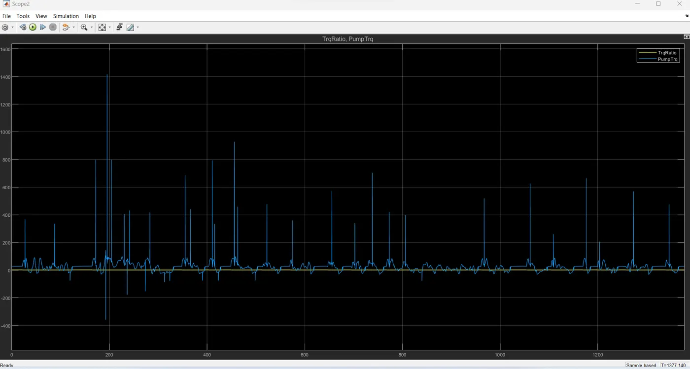
Capacity Factor , Pump Torque from Torque converter in UDDS Cyclce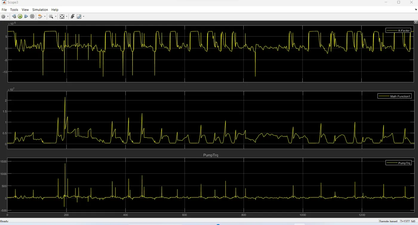
HWFET Cycle
Plots for engine , transmission input , transmission output , and wheel speed 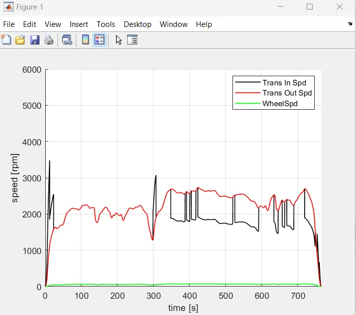
Plot engine torque, engine power, fuel rate and fuel consumption.
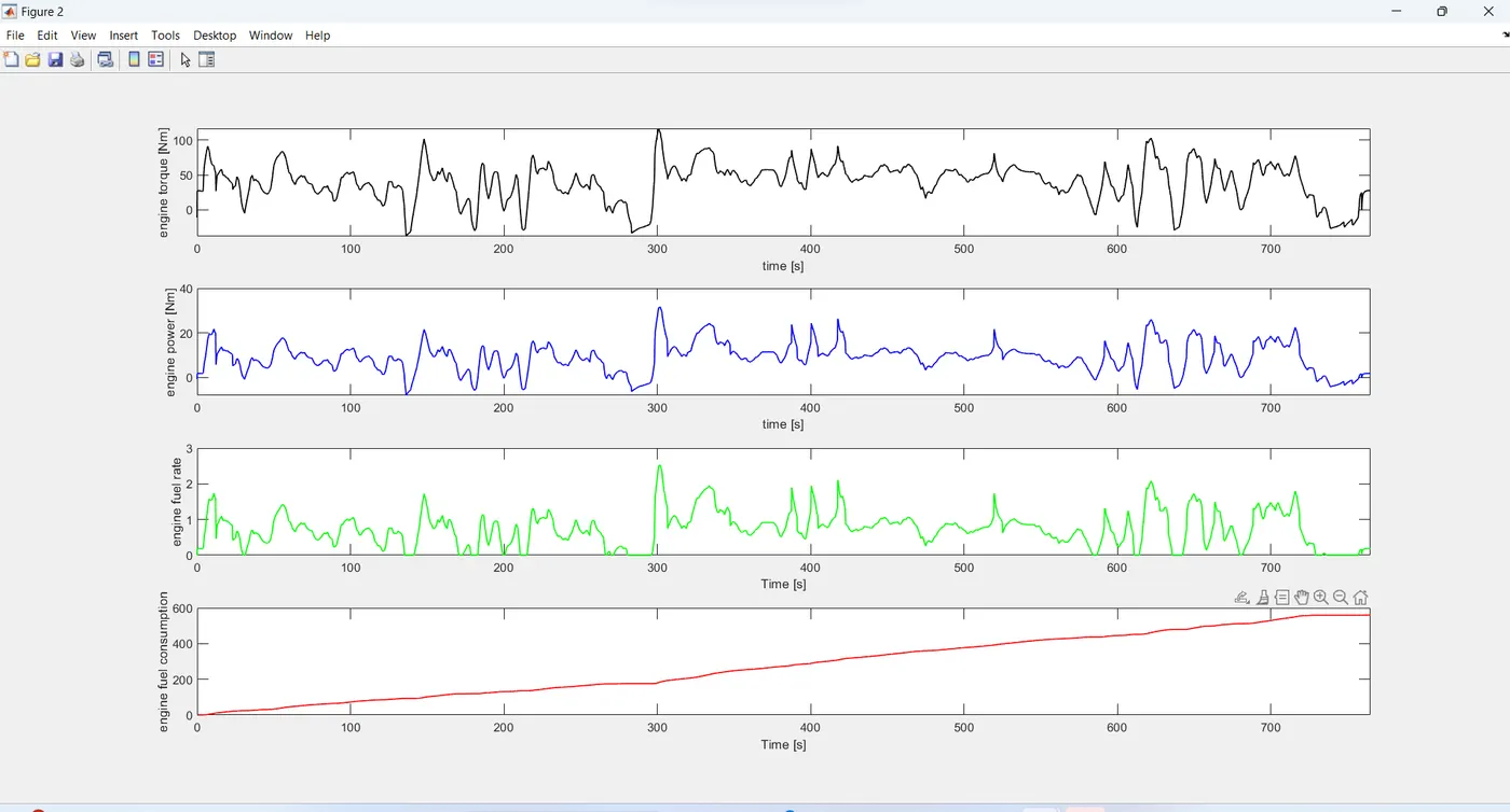
Plot accelerator and brake pedal, gear command, vehicle desired and actual speed, vehicle distance
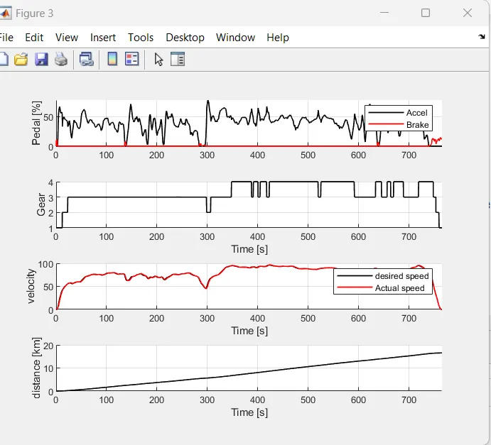
Plots for engine operating points on engine fuel map
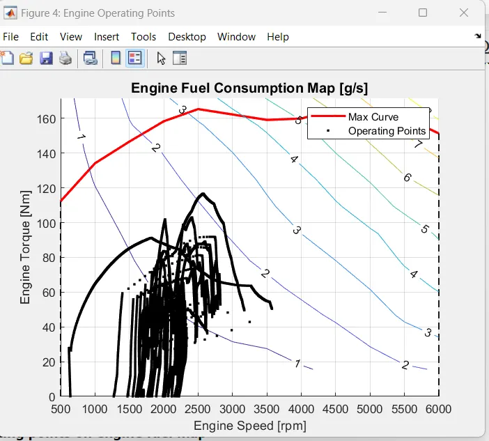
Drive cycle and Actual Velocity in HWFET Cycle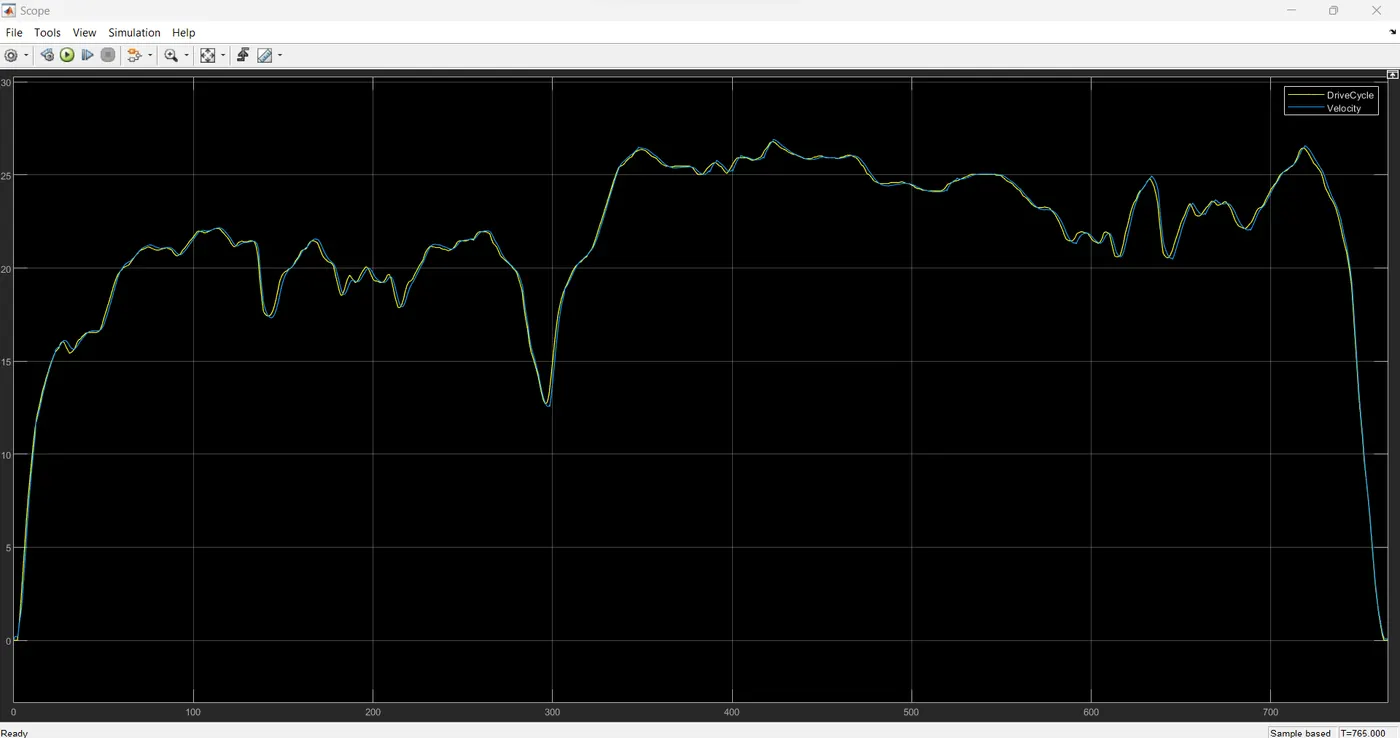
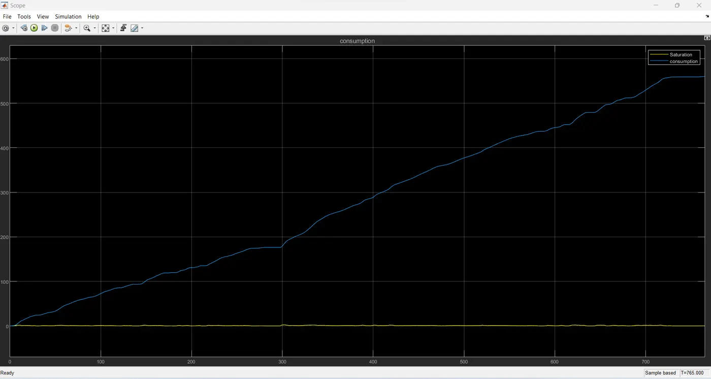
Engine Fuel flow and Fuel consumption in HWFET Cycle
Engine Torque output in HWFET Cycle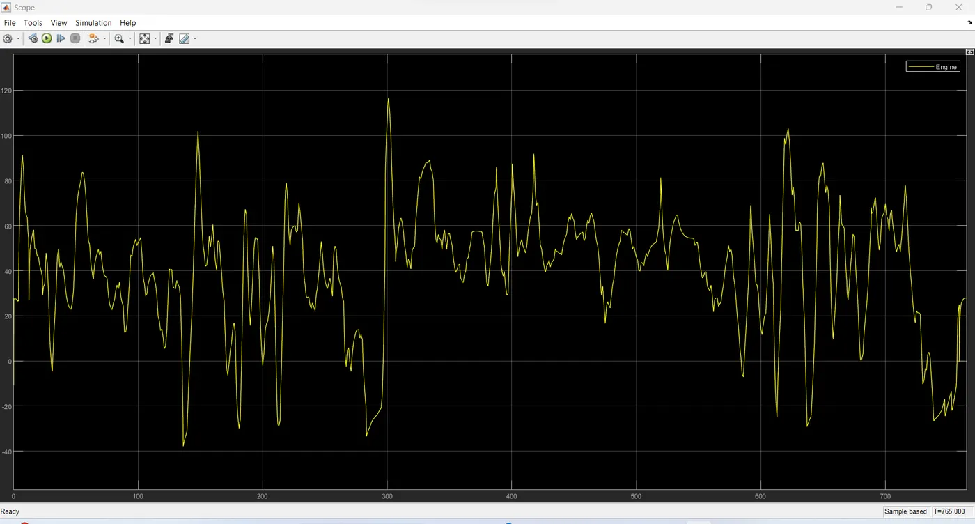
Engine Torque , Brake Torque output in HWFET Cycle 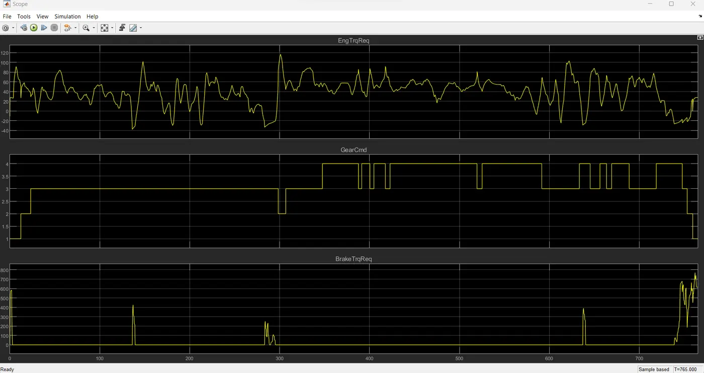
Gear Ratio , Transmission input , Transmission output in HWFET Cycle.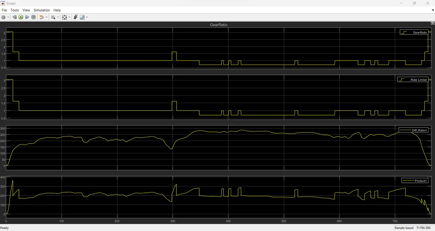
Pump speed , Turbine speed in HWFET Cycle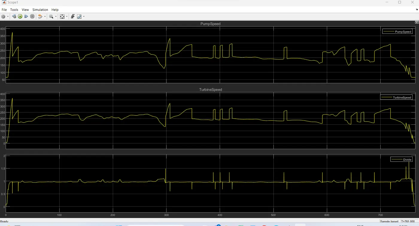
Road load , Tractive force and Accelaration in HWFET Cycle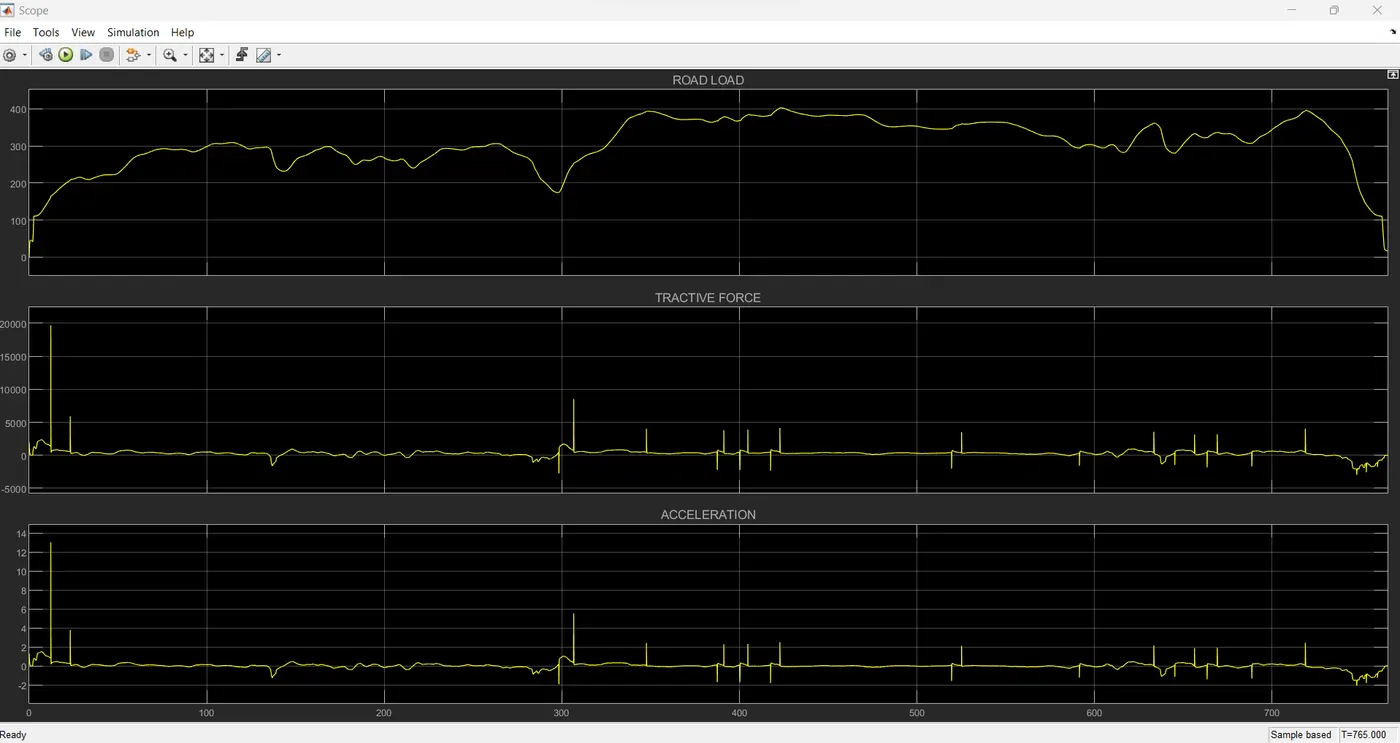
Drag resistance and Rolling resistance in HWFET Cycle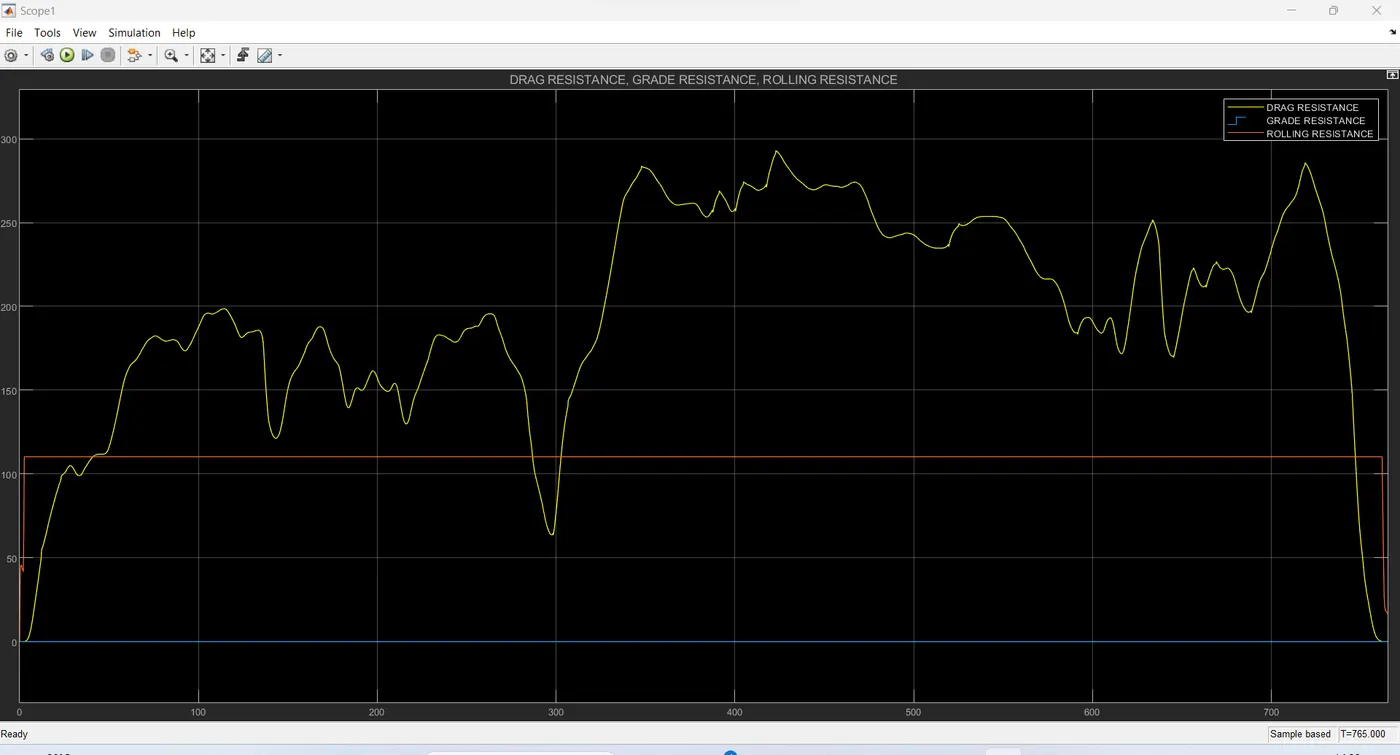
Torque ratio and Pump Torque in HWFET Cycle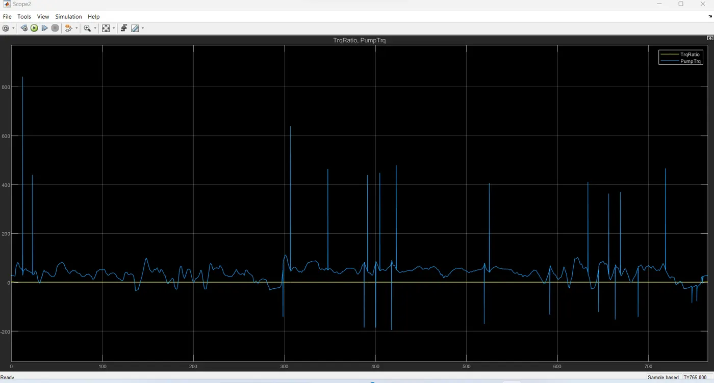
Capacity Factor , Pump Torque from Torque converter in HWFET Cyclce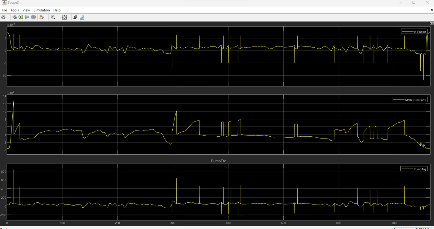
Plot the time trace for engine, transmission input, transmission output and wheel speed on one plot
The time trace plot shows the engine speed, transmission input speed, transmission output speed, and wheel speed as a function of time. The plot shows that the engine speed and transmission input speed are generally higher during the UDDS drive cycle than during the HWFET drive cycle. This is because the UDDS drive cycle includes more stop-and-go driving, which requires the engine to work harder. The transmission output speed and wheel speed are also generally higher during the UDDS drive cycle, but the difference is less pronounced.
Plot engine torque, engine power, fuel rate and fuel consumption using subplots
The engine torque, engine power, fuel rate, and fuel consumption subplots show how these variables change over time for each drive cycle. The engine torque and engine power plots show that the engine produces more torque and power during the UDDS drive cycle than during the HWFET drive cycle. This is consistent with the higher engine speed and transmission input speed observed in the time trace plot. The fuel rate and fuel consumption plots show that the engine consumes more fuel during the UDDS drive cycle than during the HWFET drive cycle. This is because the engine is working harder to meet the demands of the more aggressive UDDS drive cycle.
Plot accelerator and brake pedal, gear command, vehicle desired and actual speed, vehicle distance using subplots
The accelerator and brake pedal, gear command, vehicle desired and actual speed, and vehicle distance subplots show how these variables change over time for each drive cycle. The accelerator and brake pedal plots show that the driver uses the accelerator and brake pedals more frequently during the UDDS drive cycle than during the HWFET drive cycle. This is consistent with the more stop-and-go driving required by the UDDS drive cycle. The gear command plot shows that the transmission shifts gears more frequently during the UDDS drive cycle than during the HWFET drive cycle. This is because the engine is operating over a wider range of speeds and loads during the UDDS drive cycle. The vehicle desired and actual speed plots show that the vehicle's speed tracks the desired speed more closely during the HWFET drive cycle than during the UDDS drive cycle. This is because the UDDS drive cycle includes more aggressive acceleration and braking events. The vehicle distance plot shows that the vehicle travels a shorter distance during the UDDS drive cycle than during the HWFET drive cycle. This is because the UDDS drive cycle is shorter in duration than the HWFET drive cycle.
Plot the engine operating points on the engine fuel map
The engine fuel map plot shows the engine operating points for each drive cycle. The plot shows that the engine operates at higher speeds and loads during the UDDS drive cycle than during the HWFET drive cycle. This is consistent with the higher engine torque and engine power observed in the subplots.
Detailed explanation on plots
The plots show that the vehicle behaves differently during the UDDS and HWFET drive cycles. The UDDS drive cycle is more aggressive, with more stop-and-go driving and more aggressive acceleration and braking events. This results in higher engine speed, engine torque, engine power, fuel rate, and fuel consumption during the UDDS drive cycle. The HWFET drive cycle is less aggressive, with fewer stop-and-go driving events and less aggressive acceleration and braking events. This results in lower engine speed, engine torque, engine power, fuel rate, and fuel consumption during the HWFET drive cycle.
Comparison of UDDS and HWFET drive cycles
| Variable | UDDS | HWFET |
|---|---|---|
| Engine speed | Higher | Lower |
| Engine torque | Higher | Lower |
| Engine power | Higher | Lower |
| Fuel rate | Higher | Lower |
| Fuel consumption | Higher | Lower |
| Accelerator pedal use | More frequent | Less frequent |
| Brake pedal use | More frequent | Less frequent |
| Gear shifting | More frequent | Less frequent |
| Vehicle speed tracking | Less close | Closer |
Conclusion
The UDDS and HWFET drive cycles are two standard drive cycles used to evaluate vehicle fuel economy and emissions. The UDDS drive cycle is more aggressive than the HWFET drive cycle, and this results in higher fuel economy and emissions during the UDDS drive cycle.