Project 1

AIM:

This project's objective is to determine the vehicle's kmpl on both the urban cycle (UDDS) and the highway cycle in terms of fuel efficiency (HWFET). Also, to examine and comprehend the various aspects of how the car operates, such as the engine speed, torque, transmission speed, pedal position, gear, and distance traveled.

OBJECTIVE:

a. Tabulate the fuel economy numbers (kmpl) for UDDS and HWFET cycle. This forms the baseline numbers for comparing with the future hybrid version.

b. Plot the time trace for engine, transmission input, transmission output and wheel speed on one plot.

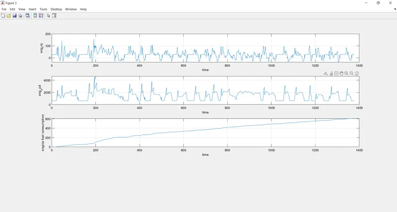
c. Plot engine torque, engine power, fuel rate and fuel consumption using subplots.

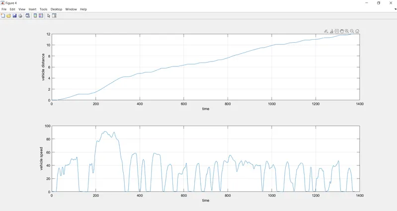
d. Plot accelerator and brake pedal, gear command, vehicle desired and actual speed, vehicle distance using subplots.

e. Plot the engine operating points on the engine fuel map.

f. Write down appropriate brief comments on each of these plots, describing the vehicle behavior throughout the drive cycle.

g. Generate the plots for both drive cycles.

THEORICITAL CONCEPTS REGARDING FORWARD ENERGY MODEL OF CONVENTIONAL VEHICLE:

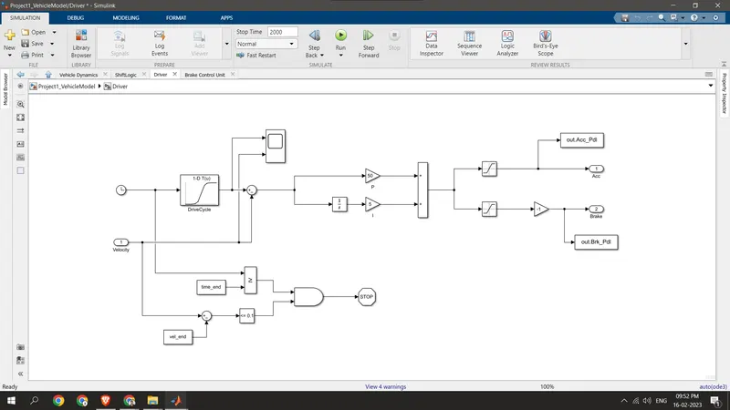
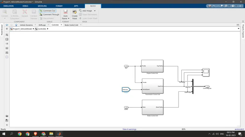
The vehicle must be controlled by a driver controller in order to follow a desired speed and establish the beginning of the computations. The controller is set up to simulate how the driver will operate the brakes or the accelerator to match the intended speed, allowing for the study of driver behavior. The controller is utilized as a component of a feedback loop to calculate the amount of energy necessary to power the vehicle.

Vehicle Energy Consumption Estimation Models:

Analytical models:

By building a vehicle model in MATLAB or Simulink, analytical models that are representational of vehicle behavior can be built. They have their foundation in basic theoretical formulae. Based on vehicle dynamics theory, a model of the vehicle's dynamics is created in order to determine how much power is needed at the wheels in order to overcome the aerodynamic drag, rolling resistance, inertia, gradient, and transmission resistances. The tractive force, which is calculated by adding the above-mentioned resistance forces, yields the necessary power.

Statistical models:

To determine the empirical correlations between the many aspects affecting a vehicle's energy usage, statistical models are created based on the study of driving data collected from real-world situations.

Computational models:

Computing models for estimating energy use mostly fall into two categories: a model based on artificial neural networks (ANN). Models that use clustering.

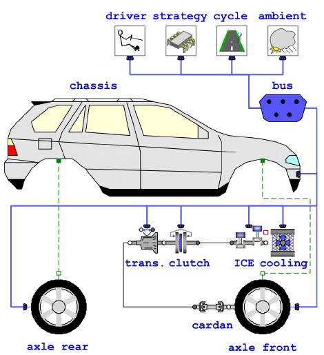
FOR UDDS:

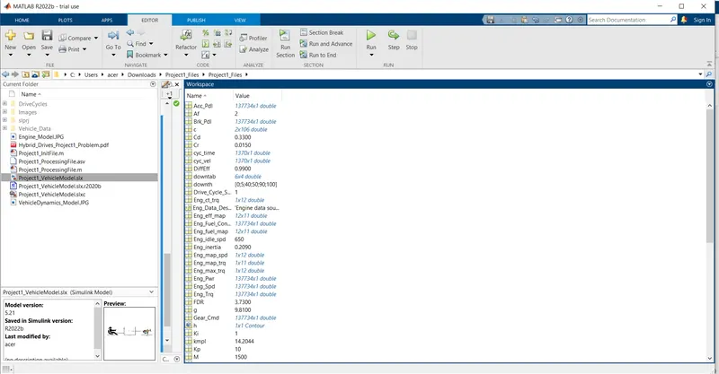
The matlab initilization file and procession file are in screeshot itself. the workspace values are also in screenshot itself.

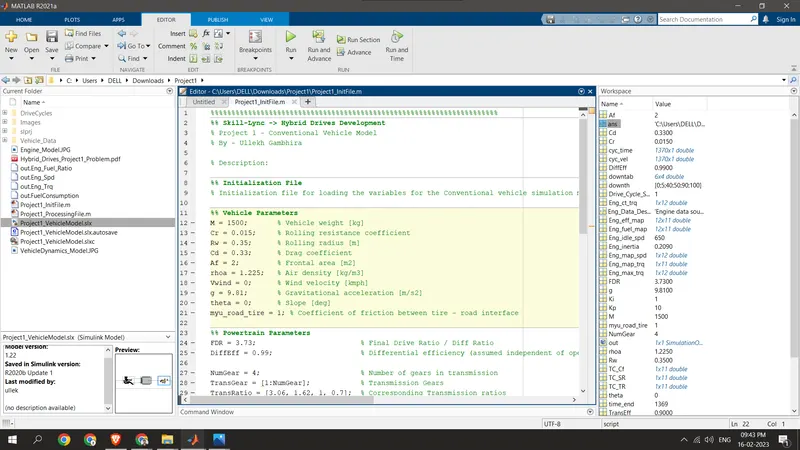
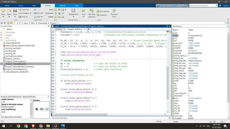
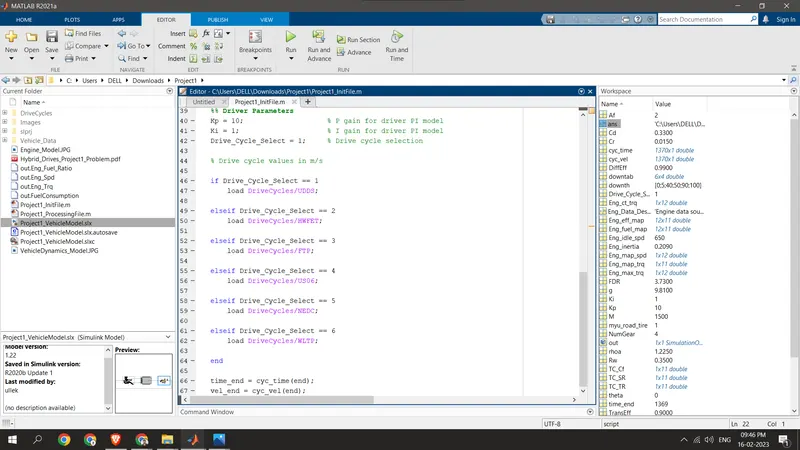
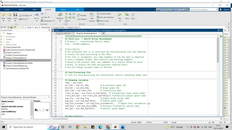
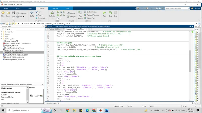
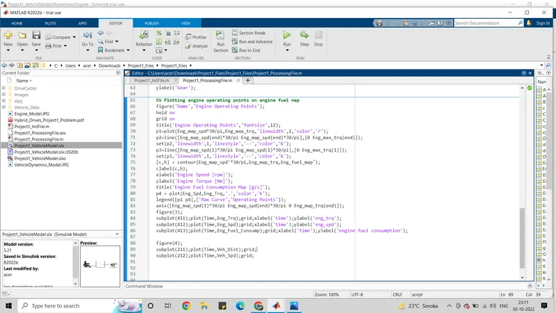
we can change the drive cycle by changing the drive cycle values:

• he Drive Cycle can be selected from this MATLAB Script, By changing the variable Drive_Cycle_Select to,

1	UDDS
2	HWFET
3	FTP
4	US06
5	NEDC
6	WLTP

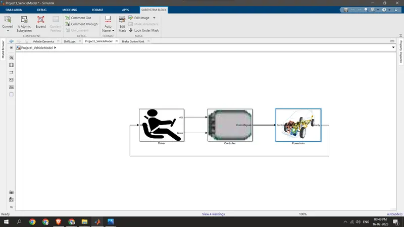
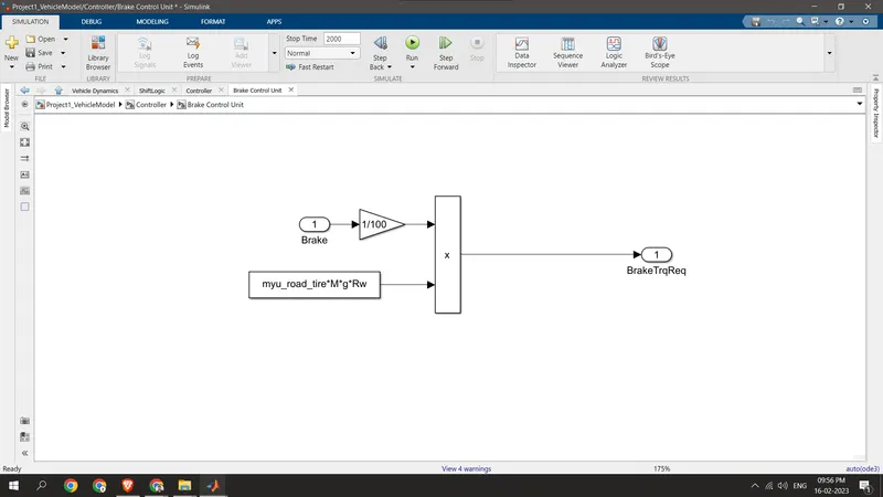
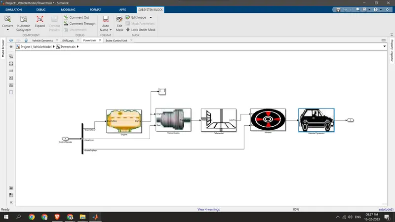
ENGINE MODEL DESCRIPTION:

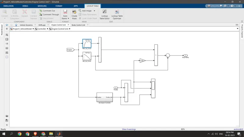
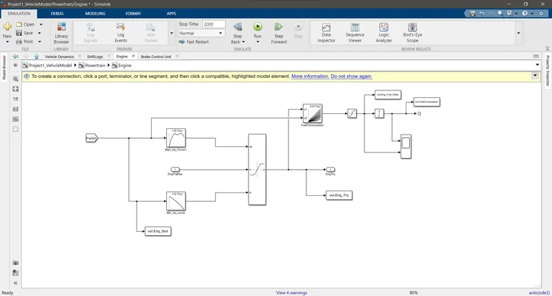
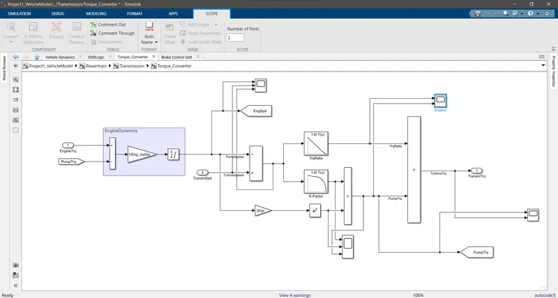
• Depending on engine speed The controller's necessary torque reaches saturation between the maximum and minimum torque curves and transfers engine torque to the transmission block.
• Based on engine speed and torque, the fuel flow rate is calculated using a 2D lookup table. The fuel consumption is then calculated using an integration of the fuel flow rate.
• The to-workspace block is used to send estimated values for fuel flow rate, fuel consumption, engine torque, and engine speed to the MATLAB workspace.
• Fuel usage and engine fuel flow rate are measured.

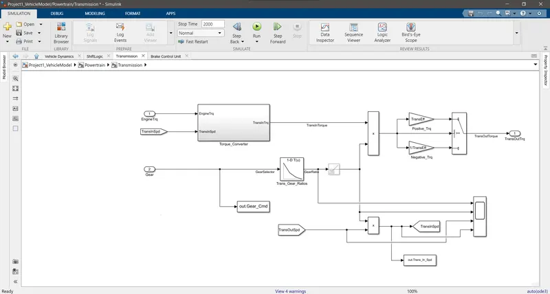
VEHICLE DYNAMICS:

Tractional force and road load are factors in this. Based on tractive force and road load, it determines how fast a vehicle should go.

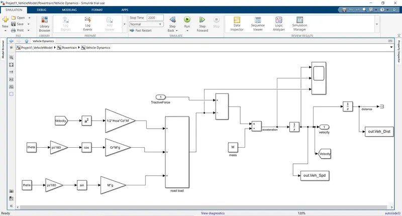
Tractive Force and Road loads are used to calculate the vehicle velocity,

Where,

ρ a - Air Density

A f - Frontal Ares

C d - Drag Coefficient

C r - Rolling Coefficient

M - Mass of Vehicle

g - Acceleration due to gravity

θ - Slope

SIMULATION RESULT OF UDDS CYCLE:

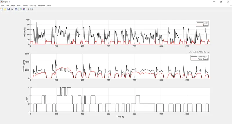
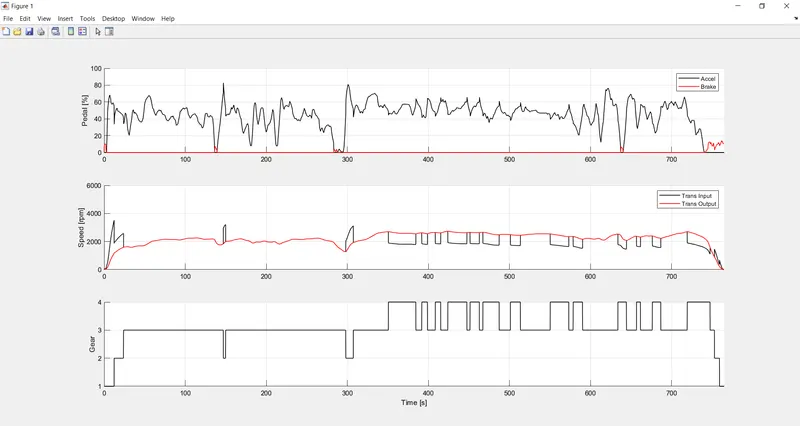
The plot below shows that as the gear is raised, the accelerator pedal rises while the brake pedal remains stationary. With each input and output transmission instant, the speed rises. When the brake pedal is in motion, speed appears to be zero.

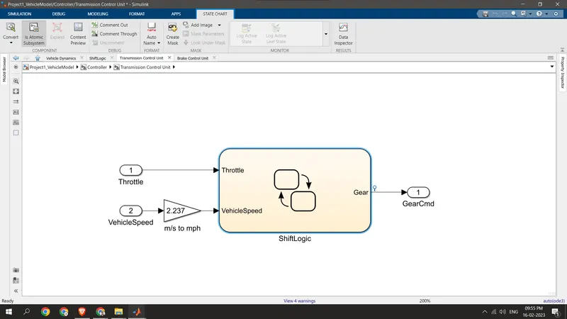
In this cycle, the vehicle only once shifts into top gear. It can only be in first or second gear for so long.

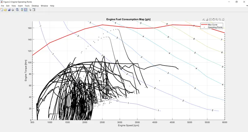
The operating points appear to be near the maximum curve. has a lower speed and torque than the UDDS driving cycle.

SIMULATION FOR HWFET CYCLE:

Overall, the ride appears to have a steady brake pedal. Most of the time, the car is in top gear, and the accelerator pedal barely moves; the brake pedal only occasionally does. For this drive cycle, the speed component shows less variation.

There is more torque generated with more engine speed. Operating points are away from the mas curve.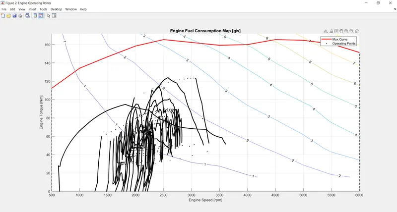

With increased torque, this drive cycle produces more power. The torque's movement exhibits a significant change. The engine speed fluctuates less frequently. Engine fuel consumption increases over time.

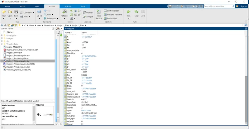
WORKSPACE FOR UDDS CYCLE: By which we can compare kmpl values :

WORKSPACE FOR HWFET CYCLE:

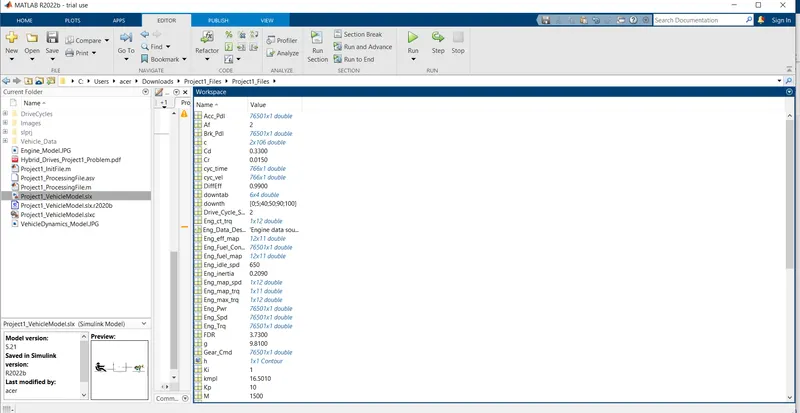
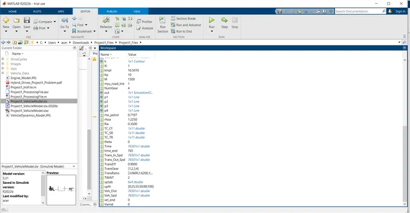
If we compare the KMPL values for UDDS and HWFET cycles, we can see that HWFET has a higher KMPL because it has lower idle losses and less frequent breaking than highway cycles, which results in higher fuel consumption.

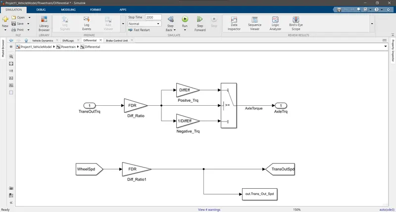
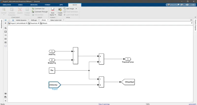
Further subsystem descriptions are not immediately necessary in our case.

CONCLUSION:

• A standard vehicle's forward energy-based fuel consumption model has therefore been successfully simulated using MATLAB and Simulink.
• Examines and comprehends aspects of vehicle operation based on engine speed, torque, transmission speed, pedal locations, gear, and distance traveled.
• Calculations after the fact were made, and the necessary graphs were successfully plotted.
• For the supplied city cycle (UDDS) and highway cycle, vehicle fuel efficiency numbers (kmpl) were determined successfully.