Project 1: A forward energy-based fuel consumption model of a conventional vehicle.

AIM

1. To Develop a forward energy-based fuel consumption model of a conventional vehicle.
2. To compute the fuel economy numbers for the given vehicle (kmpl) on the urban cycle (UDDS) and highway cycle (HWFET).
3. To analyze the vehicle operating points in terms of engine speed, torque, transmission speeds, pedal positions, gear, distance traveled, etc.

OBJECTIVE

• To build a conventional vehicle model in Simulink using blocks.
• Code in MATLAB to load all the variables required for running the model in Sumlink.
• To tabulate the fuel economy numbers (kmpl) for UDDS and HWFET cycle.
• To plot the time trace for engine, transmission input, transmission output and wheel speed on one plot.
• To plot engine torque, engine power, fuel rate and fuel consumption using subplots.
• To plot accelerator and brake pedal, gear command, vehicle desired and actual speed, vehicle distance using subplots.
• To plot the engine operating points on the engine fuel map.

THEORY

Conventional Vehicle

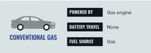
Conventional vehicles are those which use an internal combustion engine fueled by gasoline or diesel to power the wheels. Electricity is used for some accessories such as lights,starter motor,fuel pump etc.., but is not used to move the vehicle.In this vehicle the thermal energy by burning gasoline is converted in to mechanical energy.

Conventional Hybride Vehicle

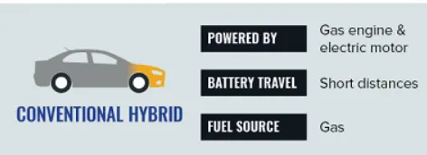
Conventional hybrids, also known as hybrid electric vehicles (HEVs), supports the internal combustion engine with electrical power produced by an on-board electric motor. The electrical system acts as a generator when a driver applies the brakes, converting kinetic energy into electrical energy that is stored in a small battery pack. The primary fuel is gasoline or diesel.

Plug-in Hybrid Vehicle

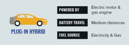
A plug-in hybrid, also called a Plug-In Hybrid Vehicle (PHEV) or an Extended Range Electric Vehicle (EREV), has a larger battery than a conventional hybrid car, and is charged by plugging into an electric outlet. Plug-in hybrids also keep a gasoline or diesel engine as a backup. After the battery energy is exhausted, the engine starts and the vehicle acts like a conventional hybrid until it is plugged in to recharge.

Battery Electric Vehicle

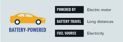
A battery-powered car, or Battery Electric Vehicle (BEV), does not have a gasoline or diesel engine and instead has an electric motor, power electronics, and a battery pack. Battery cars have a longer all-electric range than a plug-in hybrid, but they do not have a fuel backup. Just like a plug-in hybrid, battery-powered cars plug into an electric outlet to refuel.

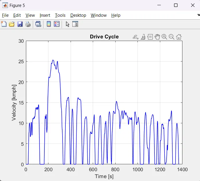
UDDS Drive Cycle (Urban Dynamometer Drive Schedule)

The UDDS (Urban Dynamometer Driving Schedule) drive cycle is a standardized test procedure used to evaluate the emissions and fuel economy of vehicles. It is one of several driving cycles that have been developed by the U.S. Environmental Protection Agency (EPA) to represent real-world driving conditions. The UDDS drive cycle is designed to simulate the types of driving conditions encountered in an urban setting, such as stop-and-go traffic and short trips.

The UDDS drive cycle consists of a series of stops and starts, accelerations and decelerations, and steady-state driving segments. The cycle begins with a cold start, where the vehicle is allowed to idle for a period of time to allow the engine and catalytic converter to warm up. This is followed by a series of acceleration and deceleration events, designed to simulate the stop-and-go nature of urban driving. The cycle also includes several steady-state driving segments at different speeds, ranging from 20 to 60 mph.

The UDDS drive cycle is typically run on a chassis dynamometer, which is a device that simulates the resistance of driving on a road by applying a load to the vehicle's wheels. The dynamometer is used to measure the vehicle's emissions and fuel consumption during the test. The UDDS drive cycle is used to test light-duty vehicles, including passenger cars, pickup trucks, and vans. It is typically run in conjunction with other driving cycles, such as the Highway Fuel Economy Test (HFET) and the Cold Start FTP (Federal Test Procedure).

The UDDS drive cycle is an important tool for evaluating the environmental performance of vehicles. It allows manufacturers to compare the emissions and fuel economy of different vehicles under controlled conditions and helps regulators ensure that vehicles meet emissions standards. It is also used by consumers to compare the fuel efficiency of different vehicles and make informed purchasing decisions.

Overall, the UDDS drive cycle is a valuable tool for evaluating the environmental performance of vehicles and helps ensure that vehicles meet emissions standards. It is an important part of the vehicle testing and certification process, and is used by manufacturers, regulators, and consumers to evaluate the performance of vehicles.

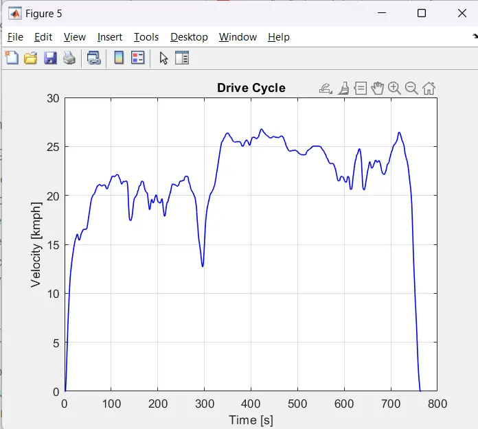
HWFET Drive Cycle (Highway Fuel Economy Test)

The Highway Fuel Economy Test (HFET) drive cycle is a standardized test procedure used to evaluate the fuel economy of vehicles. It simulates driving conditions encountered on the highway and consists of acceleration and deceleration events, as well as steady-state driving segments at different speeds. The HFET drive cycle is typically run on a chassis dynamometer, which measures the vehicle's fuel consumption during the test. The cycle is used to test light-duty vehicles and is an important tool for evaluating the fuel efficiency of vehicles. It is used by manufacturers, regulators, and consumers to compare the fuel efficiency of different vehicles and make informed purchasing decisions.

The HFET drive cycle consists of a series of acceleration and deceleration events, as well as steady-state driving segments at different speeds. The cycle begins with a cold start, where the vehicle is allowed to idle for a period of time to allow the engine and catalytic converter to warm up. This is followed by a series of acceleration and deceleration events, designed to simulate the stop-and-go nature of urban driving. The cycle also includes several steady-state driving segments at different speeds, ranging from 35 to 60 mph.

The Federal Test Procedure (FTP)

The FTP drive cycle consists of a series of acceleration and deceleration events, as well as steady-state driving segments at different speeds. The cycle is typically run on a chassis dynamometer, which is a device that simulates the resistance of driving on a road by applying a load to the vehicle's wheels. The dynamometer is used to measure the vehicle's emissions and fuel consumption during the test. The FTP drive cycle is used to test light-duty vehicles, including passenger cars, pickup trucks, and vans, and is an important tool for evaluating the environmental performance of vehicles. It is used by manufacturers, regulators, and consumers to compare the emissions and fuel efficiency of different vehicles and make informed purchasing decisions.

New European Driving Cycle (NEDC)

The New European Driving Cycle (NEDC) is a standardized test procedure used to evaluate the emissions and fuel economy of vehicles. It was developed by the European Union (EU) to represent real-world driving conditions in Europe and was used as the basis for emission and fuel economy regulations in the EU.The NEDC was used as the primary test cycle for emission and fuel economy regulations in the EU until it was replaced by the Worldwide harmonized Light vehicles Test Procedure (WLTP) in 2017. The NEDC was criticized for being too lenient and not accurately reflecting real-world driving conditions, leading to the development of the WLTP, which is a more representative and stringent test cycle. The NEDC is no longer used for regulatory purposes, but it is still widely used for vehicle testing and certification. It is an important tool for evaluating the environmental performance of vehicles and is used by manufacturers, regulators, and consumers to compare the emissions and fuel efficiency of different vehicles and make informed purchasing decisions.

There are two types of Energy modeling approches:

1. Forward energy-based fuel consumption model
2. Backward Energy-based fuel consumption model

1. Forward energy-based fuel consumption model

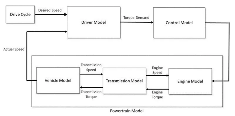
The forward modelling is also known as cause-effect, engine-to-wheel or rear-to-front method. The direction of calculation is the same as the direction of positive power flow which is from engine to wheels.

A forward-facing vehicle model feactures a driver model that provides torque demand in the form of a desiered ICE torque and brake torque, to meet the speed trace from a drivecycle.A basic driver model typically uses one or more Proportional- Intrgral (PI) controllers to achieve the torque demand, with reference to the desiered speed trace.The torque produced by the ICE propagates through the transmission and final drive ratios, before ending up as torque applied at the wheels. This is then exerted to the vehicle mass via force on the tyre contact patch. The vehicle speed that results from the applied force is propagated back through the drivetrain, and returns to the ICE as angular velocity at the crankshaft. Brake torque is applied directly at the wheels.

This model can be used to compare the fuel efficiency of different vehicles, or to identify opportunities for improving the fuel efficiency of a particular vehicle. For example, if you are trying to improve the fuel efficiency of a vehicle, you could modify its design or driving behavior to reduce its energy consumption, and then use the forward energy-based fuel consumption model to estimate the resulting improvement in fuel efficiency.

2. Backward Energy-based fuel consumption model

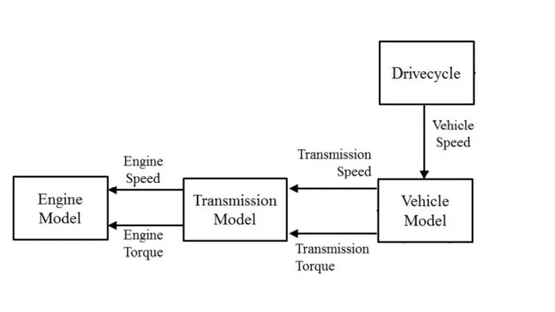
Backward-facing (quasi-static) vehicle model, the ability of the vehicle model to meet the demands of the drivecycle is the principle assumption of a backward-facing model.Based on the speed trace, the resultant force at the tyre contact patch is calculated, where it is converted into wheel torque and propagated back to the ICE via the drivetrain, along with angular velocity. As a result, there is no driver model present. With both speed and torque imposed onto the powertrain components, a backward-facing model can also be considered as non-causal (physically non-realisable).During the optimisation routine, the powertrain component sizing is determined by the ability of the component to address both the speed and torque imposed on the component (i.e. the power requirements).
Backward-facing models rely on efficiency maps that were created based on torque and speed data, and usually produced during steady-state real world testing. This results in the calculation being relatively simpler than forward-facing models (essentially lookup tables instead of state equations),and can therefore be run over relatively larger time steps.Unfortunately, the very nature of using steady state maps hinders the performance of backward-facing models when it comes to representing dynamic effects.


PROGRAM CODE

% Conventional Vehicle Model
close all
clear all
clc

% Vehicle parameters
M = 1500;          % Vehicle weight [kg]
Cr = 0.015;        % Rolling resistance coefficient
Rw = 0.35;         % Rolling radius [m]
Cd = 0.33;         % Drag coefficient
Af = 2;            % Frontal area [m2]
rhoa = 1.225;      % Air density [kg/m3]
Vwind = 0;         % Wind velocity [kmph]
g = 9.81;          % Gravitational acceleration [m/s2]
theta = 0;         % Slope [deg]
myu_road_tire = 1; % Coefficient of friction between tire - road interface

% Powertrain Parameters 
FDR = 3.73;                         % Final Drive Ratio / Diff Ratio
DiffEff = 0.99;                     % Differential efficiency

NumGear = 4;                        % Number of gears in transmission
TransGear = 1:NumGear;              % Transmission Gears
TransRatio = [3.06, 1.62, 1, 0.7];  % Corresponding Transmission ratios
TransEff = 0.90;                    % Transmission efficiency 

TC_SR = [0, .5, .6, .7, .8, .87, .92, .94, .96, .97, 1];   % Torque Converter Speed Ratio (Matlab default) -> TurbSpd/PumpSpd  
TC_TR = [2.232, 1.5462, 1.4058, 1.2746, 1.1528, 1.0732, 1.0192, 1, 1, 1, 1];   % Torque Converter Torque Ratio (Matlab default) -> TurbTrq/PumpTrq
TC_Cf = 1e-4 * [.72558, .66322, .63463, .59042, .51331, .4144, .29287, .22444, .12186, .04386, 0]; % Torque Converter Capacity Factor (Matlab default) -> PumpTrq/PumpSpd^2 [Nm/rpm^2]

load Vehicle_Data/Engine_data_1_9L_Saturn_95kW;
load Vehicle_Data/Trans_Shift_map;

% Driver Parameters
Kp = 10;                    % P gain for driver PI model
Ki = 1;                     % I gain for driver PI model
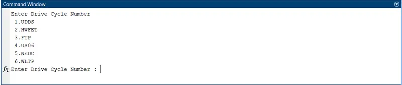
fprintf('Enter Drive Cycle Numbern 1.UDDSn 2.HWFETn 3.FTPn 4.US06n 5.NEDCn 6.WLTPn'); % Drive cycle selection
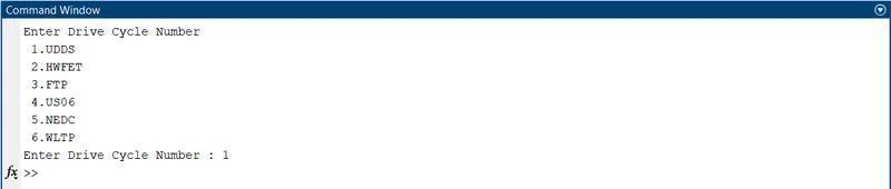
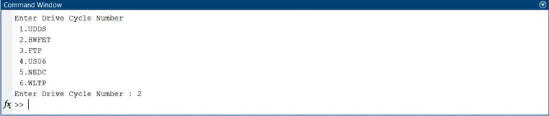
Drive_Cycle_Select =input('Enter Drive Cycle Number : ');    

% Drive cycle values in m/s

if Drive_Cycle_Select == 1
    load DriveCycles/UDDS;
    
elseif Drive_Cycle_Select == 2
    load DriveCycles/HWFET;
    
elseif Drive_Cycle_Select == 3
    load DriveCycles/FTP;
    
elseif Drive_Cycle_Select == 4
    load DriveCycles/US06;
    
elseif Drive_Cycle_Select == 5
    load DriveCycles/NEDC;
    
elseif Drive_Cycle_Select == 6
    load DriveCycles/WLTP;
 
end

time_end = cyc_time(end);
vel_end = cyc_vel(end);

CODE EXPLAINATION

• The program begins by clearing and closing the memory using close all clear all clc functions.
• Then the vehicle parameters and constants were initilized.
• The engine datas and the gear shift datas were loaded to Matlab using the load command.
• Then the driver parameters proportional and integral cofficients were decelared.
• Then using the fprintf() the different drive cycles were showen and using the input() command the user input of the required drive cycle is recieved.
• Again using load command the particular drive cycle data selected by user is loaded in Matlab and the end time and end velocity of vehicle is obtained.

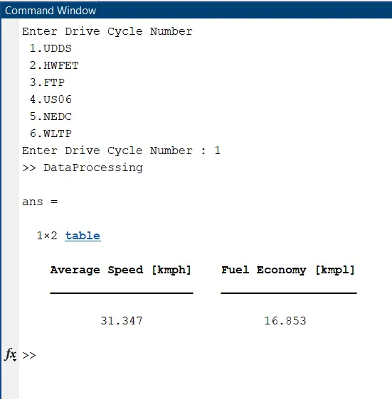
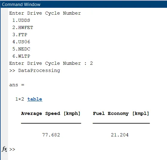
COMMAND WINDOW

Taking user input

WORKSPACE

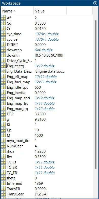
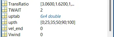
SIMULINK MODEL

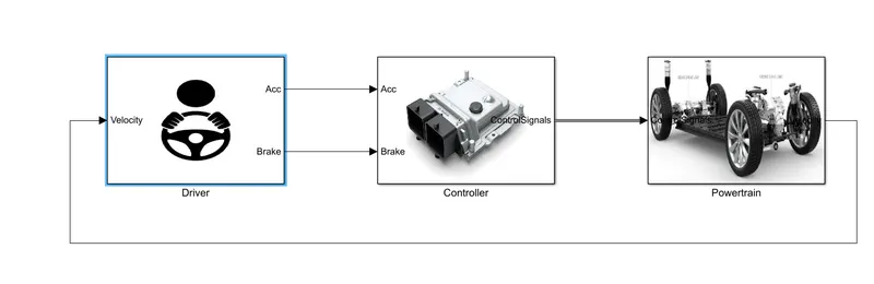
The Simulink model for the convection vehicle consist of using 3 main subblocks: driver model, control model and powertrain block.The model developed is capable to simulate the vehicle on different drive cycles like UDDS, HWFET, FTP, US06,NEDC and WLTP.

The Driver model

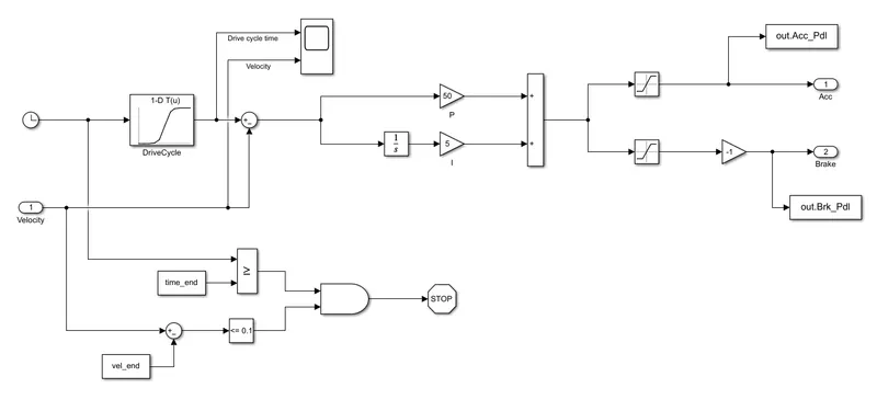
• The Driver Model is a basicially a Proportional Integral (PI) controller that generates accelerator and brake pedal outputs to match the desired and actual vehicle speeds as per the drive cycle.
• The PI controller controls the error between the required drive cycle velocity and actual vehicle velocity.
• This model takes in the vehicle velocity and gives the accleration and brake output to controller.

Controller Model

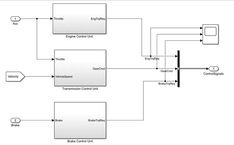
The Controller consists of 3 sub blocks : Engine control unit, Transmission control unit and Brake control unit.This model recieves the accleration and brake values and gives out engine torque,Gear and Brake torque as per requirement of the drive cycle.

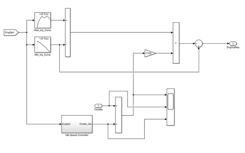
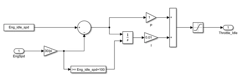
Engine control unit : This block takes in the throttle and compares the engine speed with maxium torque and minium torque curves of lookup table and gives out the engine required torque.It also controls the idle speed and gives out the idle throttle from the idle throttle controller.

Idle Speed Controller

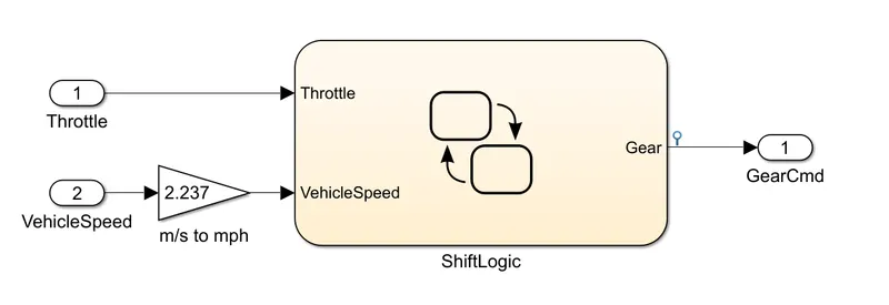
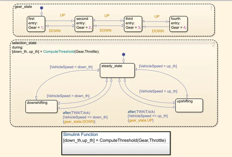
Transmission Control Unit: The transmission control block controls the gear shifting of vehicle using the State flow .The model takes in throttle and vehicle speed and shifting of gears up and down is done automatically and gives the gear command as output.

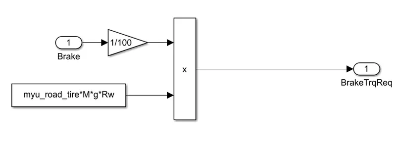
Brake control unit: It combines the load on road with the tyre in contact along with the braking applied and gives out the required brake torque as per the drive cycle.

Powertrain Model

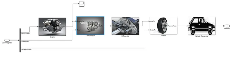
Its the block where the engine power is converted for motion at the wheels.This block recieves control signals of Torqure required by engine, gear command and brake torque depeneding on which the output on wheels were controlled.It compraises of Engine,Transmission,Differential,Wheels and the vehicle dynamics.

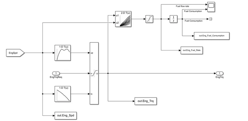
Engine block: Based on the torque request from the controller it checks whether is between max torque and min torque using a dynamic saturation block and gives the engine torque output.

It also calculate the fuel consumption by taking the engine speed and torque with the help of 2D lookup tabe.

Using the To Workspace block the fuel flow rate, engine fuel consumption, Engine torque and Engine Speed are transfered to workspace.

Transmission: Transmission block takes in the engine torque and gear command and with automatic transmission it gives out the transmission torque to the differential.

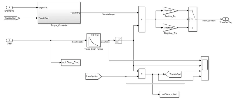
Torque Converter: The engine dynamics calculate the accleration and speed of the engine based on the net torque acting on the engine inerrtia.It gives out the transmission input torque which is then multiplied with the gear commanded to gives put the transmission torque.

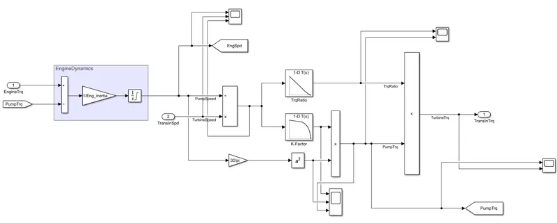
Differential: The transmission output torque from the transmission block is multiplied with the differential ratio and using a swith block the axle torque is obtained and provided to wheels.Also the transmission output speed is obtained by multiplying wheel speed with the differential ratio.

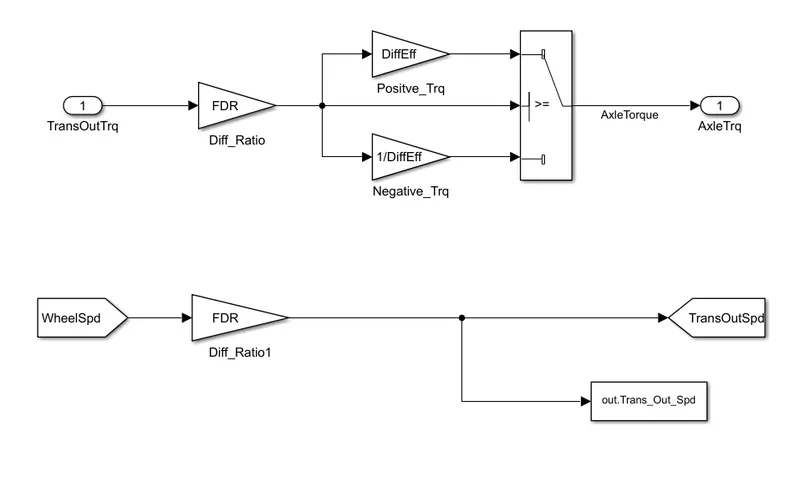
Wheels: The block takes in the axle torque from the differential block and the brake torque signal from the controller and it is then added and multiplied with the Rolling radius of the wheel.This will provide the Tractive force on the wheel.

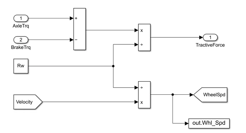
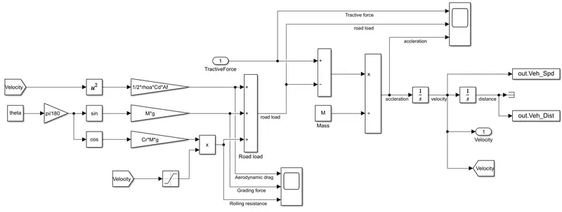
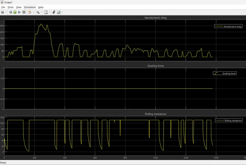
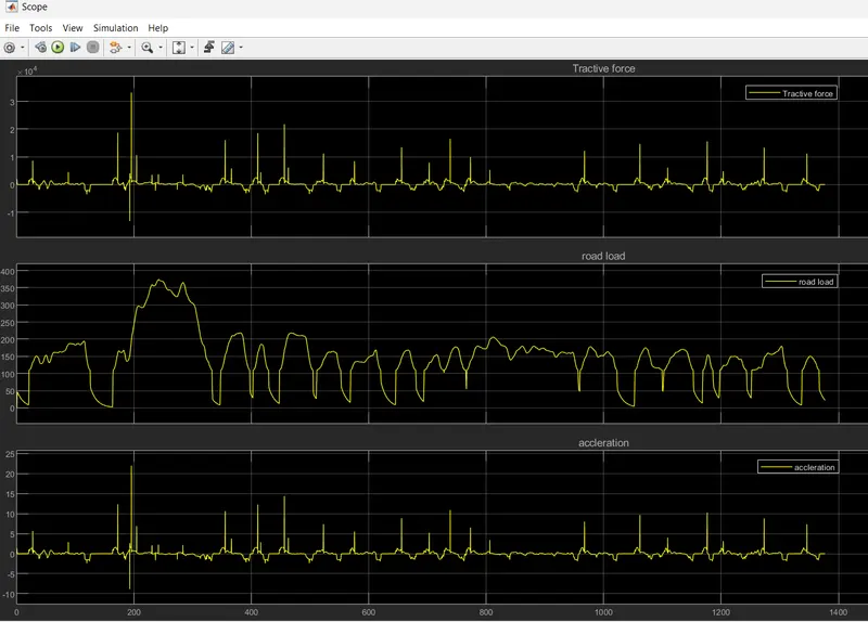
Vehicle Dynamics : In vehicle dynamics the tractive force is combined with the various resistances such as rolling resistance,aerodynamic drag, grading force which makes up the road load.It is then divided with the mass of the vehicle and integrated to get the velocity of the vehicle.

OUTPUT

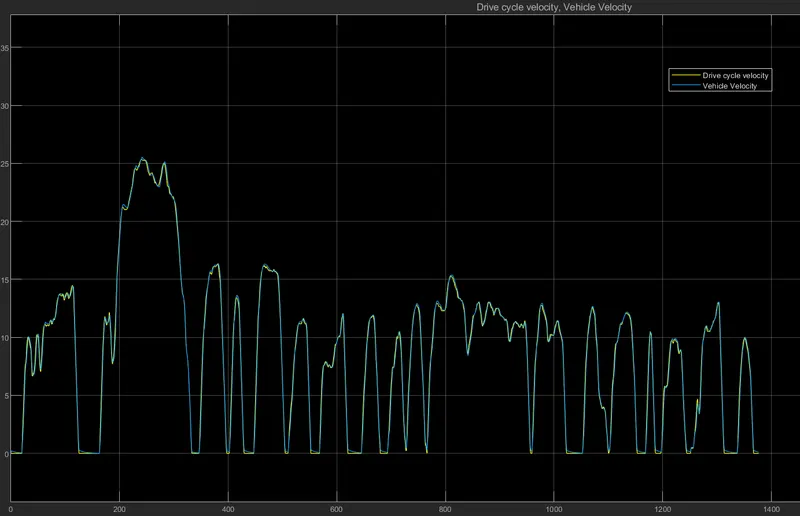
Drive cycle velocity vs Vehicle velocity of UDDS drive cycle from driver block

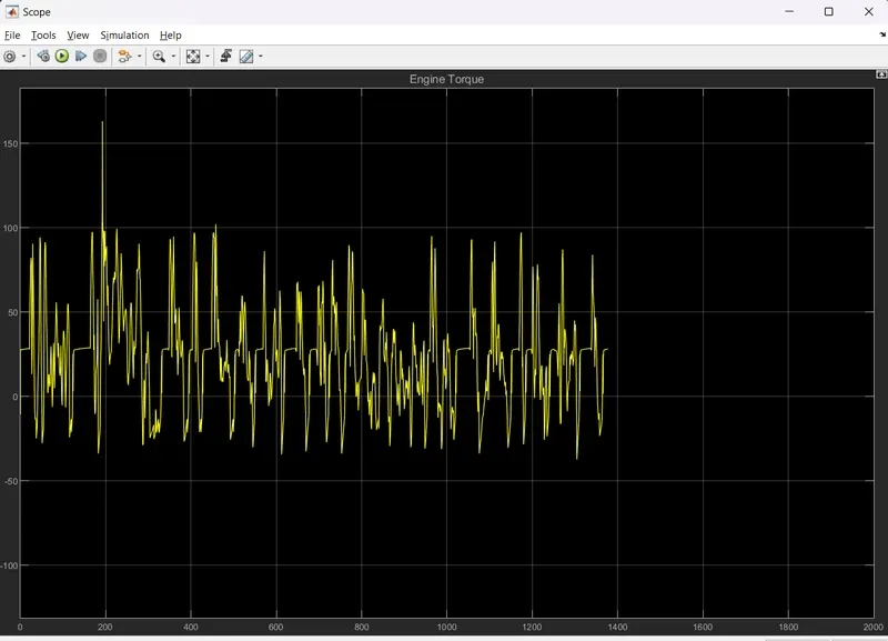
Engine Torque output in UDDS Cycle

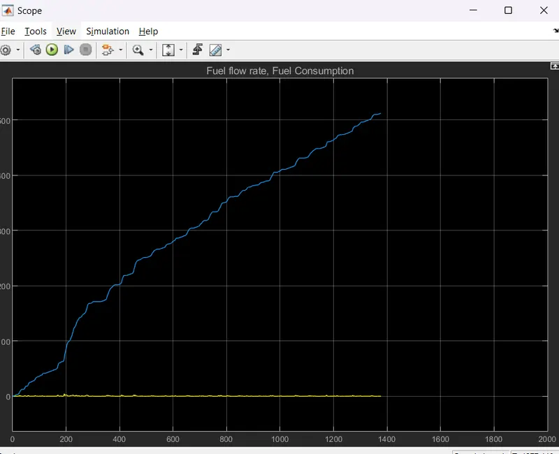
Fuel Flow rate and Fuel Consumption from Engine block in UDDS cycle

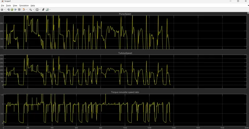
Pump Speed,Turbine Speed ,Torque converter speed ratio from Transmission block in UDDS Cycle

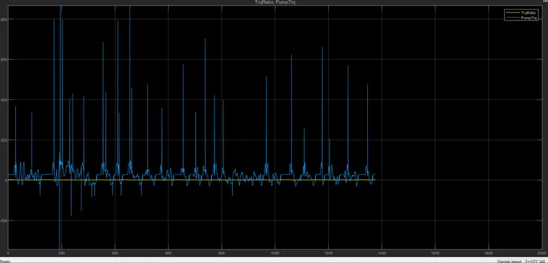
Torque ratio and Pump Torque from Transmission block in UDDS Cycle

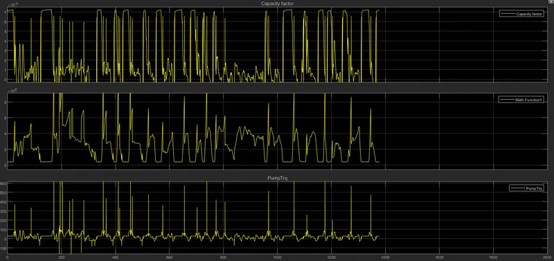
Capacity Factor Pump Torque from Transmission block in UDDS Cycle

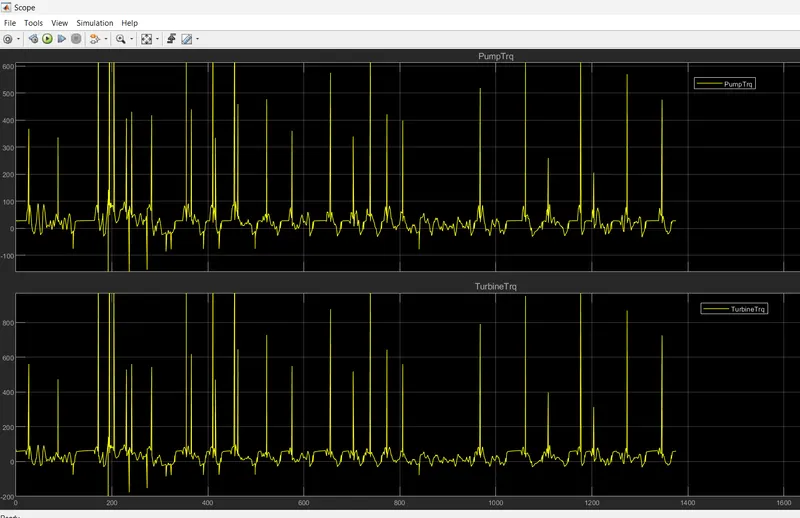
Pump Torque and Turbine Torque from Transmission block in UDDS Cycle

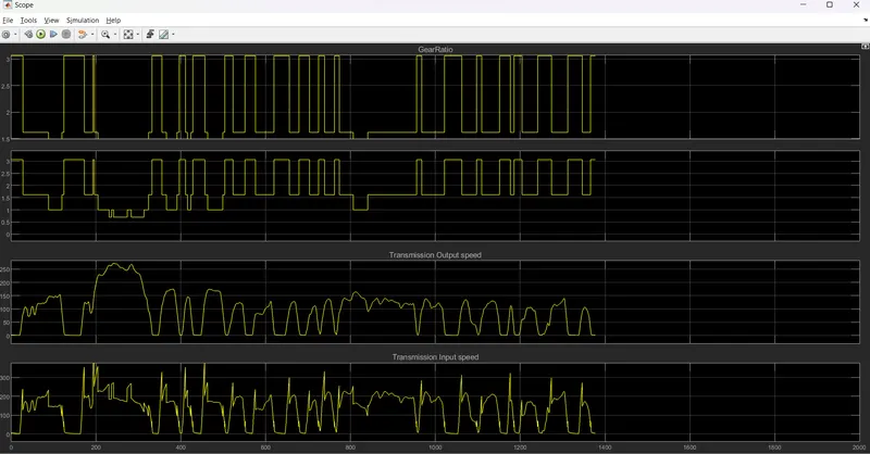
Gear ratio, Transmission Input and Transmission Ouput Speed from Transmission block in UDDS cycle.

Aerodynamic drag,Grading force and Rolling resistance VS Time from Vehicle dynamic block in UDDS Cycle

Tractive force,Road load and Accleration VS Time From vehicle dynamic block in UDDS Cycle

OUTPUT (HWFET Drive Cycle)

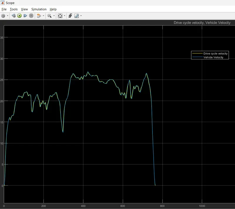
Drive cycle velocity vs Vehicle velocity of HWFET drive cycle from driver block

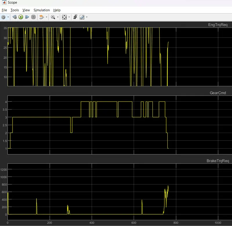
Engine Torque,Gear command and Brake Torque From Controller block for HWFET Cycle

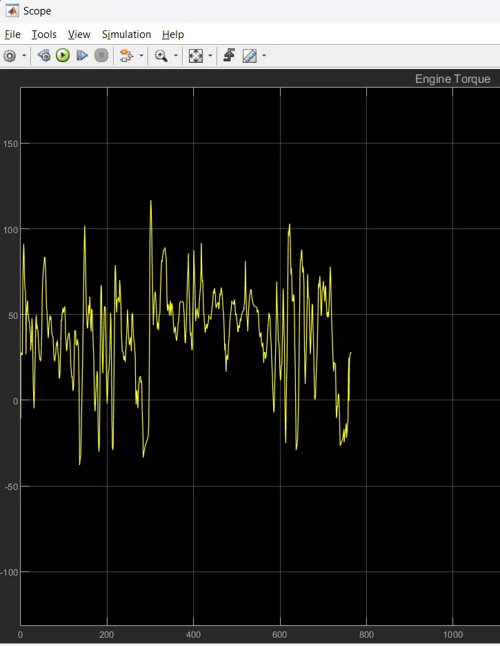
Engine Torque output in HWFET Cycle

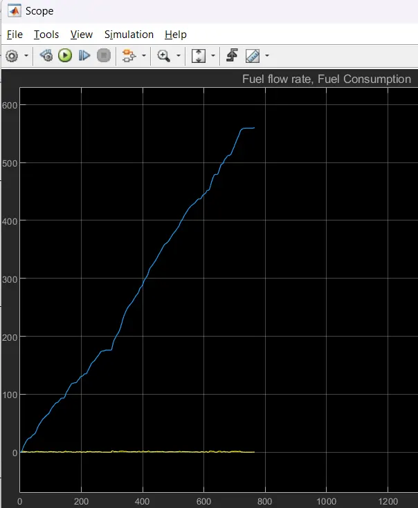
Fuel Flow rate and Fuel Consumption from Engine block in HWFET cycle

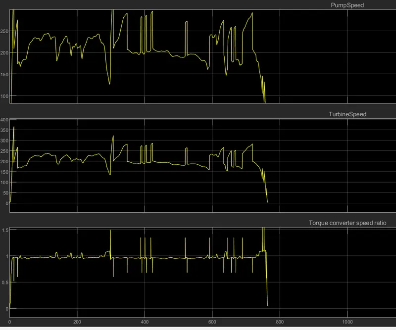
Pump Speed,Turbine Speed ,Torque converter speed ratio from Differential block in HWFET Cycle.

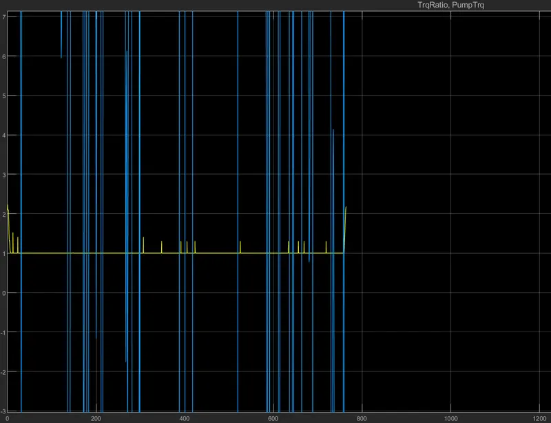
Torque ratio and Pump Torque from Differential block in HWFET Cycle.

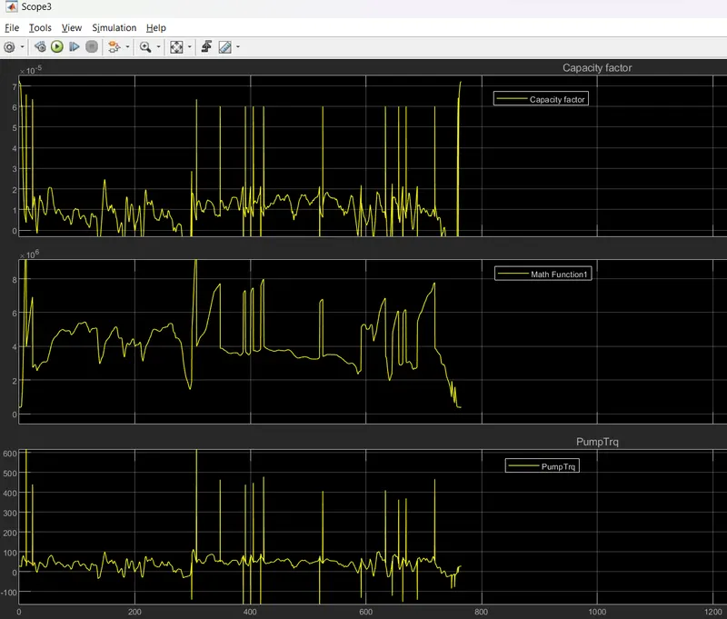
Capacity Factor Pump Torque from Differential block in HWFET Cycle.

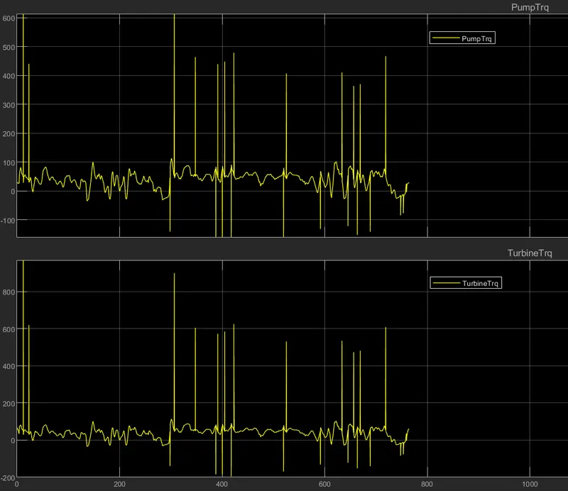
Pump Torque and Turbine Torque from Transmission block in HWFET Cycle

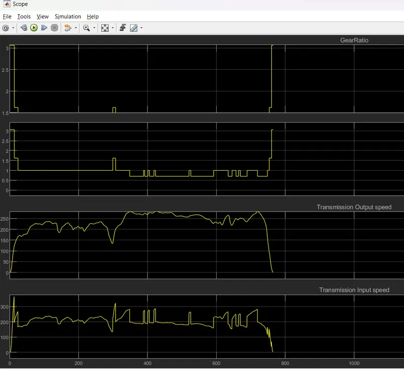
Gear ratio, Transmission Input and Transmission Ouput Speed from Transmission block in HWFET cycle.

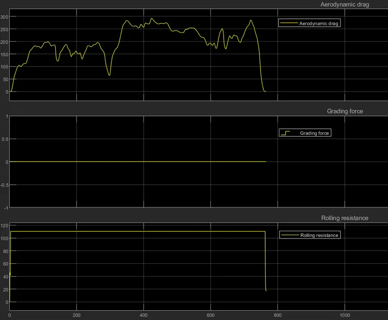
Aerodynamic drag,Grading force and Rolling resistance VS Time from Vehicle dynamic block in HWFET Cycle.

Tractive force,Road load and Accleration VS Time From vehicle dynamic block in HWFET Cycle

Post-Processing Conventional Vehicle simulation model

PROGRAM CODE

% Renaming & Defining Variables
Time = out.tout;
Acc_Pdl = out.Acc_Pdl;                      % Accelerator pedal [%]
Brk_Pdl = out.Brk_Pdl;                      % Brake pedal [%]
Gear_Cmd = out.Gear_Cmd;                    % Transmission gear
Trans_In_Spd = out.Trans_In_Spd*30/pi;      % Transmission input speed [rpm]
Trans_Out_Spd = out.Trans_Out_Spd*30/pi;    % Transmission output speed [rpm]
Eng_Trq = out.Eng_Trq;                      % Engine brake torque [Nm]
Eng_Spd = out.Eng_Spd*30/pi;                % Engine speed [rpm]
Eng_Fuel_Consump = out.Eng_Fuel_Consumption;% Engine fuel consumption [g]
Veh_Dist = out.Veh_Dist/1000;               % Distance traveled by vehicle [km]
Veh_Spd = out.Veh_Spd*18/5;                 % Vehicle speed [kmph]
Whl_Spd=out.Whl_Spd*30/pi;                  % Wheel speed [rpm]
Eng_Fuel_Rate=out.Eng_Fuel_Rate;            % Engine fuel rate [%]
Desiered_velocity=cyc_vel*18/5;             % Desiered velocity as per drive cycle [kmph]
% Data analysis
Eng_Pwr = Eng_Spd*pi/30*Eng_Trq/1000;                        % Engine brake power [kW]
rho_petrol = 0.7197;                                         % Density of petrol [kg/L]
kmpl = Veh_Dist(end)/(Eng_Fuel_Consump(end)/1000/rho_petrol);% Fuel economy [kmpl] 

% Tabulation of Average speed and Fuel econony
Avg_speed = sum(Veh_Spd)/length(Veh_Spd);
table(Avg_speed,kmpl(:,1),'VariableNames',{'Average Speed [kmph]','Fuel Economy [kmpl]'})

% Plotting 

% Time trace for engine, transmission input, transmission output and wheel speed
figure(1)
hold on
grid on
plot(Time,Trans_In_Spd,'LineWidth',1,'Color','m');
plot(Time,Trans_Out_Spd,'LineWidth',1,'Color','k');
plot(Time,Whl_Spd,'LineWidth',1,'Color','g');
xlabel('Time [s]');
ylabel('Speed [rpm]');
xlim([0, Time(end)]);
legend('Transmission Input Speed','Transmission Output Speed','Wheel Speed');

% Engine torque, engine power, fuel rate and fuel consumption
figure(2)
subplot(2,2,1);
plot(Eng_Trq,'linewidth',1,'color','1,0.7,0.3');
xlabel('Time [s]');
ylabel('Engine Torque [Nm]');
title('Engine Torque VS Time');
grid on;
subplot(2,2,2)
plot(Eng_Pwr,'linewidth',1,'color','0.8,0.3,0.6');
xlabel('Time [s]');
ylabel('Engin Power [Kw]');
title('Engine power VS Time');
grid on;
subplot(2,2,3)
plot(Time,Eng_Fuel_Rate,'linewidth',1,'color','0.4,0.7,0.5');
xlabel('Time [s]');
ylabel('Engin fuel rate [%]');
title('Fuel rate VS Time');
grid on;
subplot(2,2,4)
plot(Time,Eng_Fuel_Consump,'linewidth',1,'color','0.6,0.2,1')
xlabel('Time [s]');
ylabel('Fuel Consumption [g]');
title('Fuel Consumption VS Time');
grid on;

% Accelerator and brake pedal, gear command, vehicle desired and actual speed, vehicle distance
figure(3)
subplot(4,1,1)
hold on
grid on
plot(Time, Acc_Pdl, 'linewidth', 1, 'Color', 'g');
plot(Time, Brk_Pdl, 'linewidth', 1, 'Color', 'b');
ylabel('Pedal [%]');
xlim([0, Time(end)]);
legend('Accel','Brake');
subplot(4,1,2)
hold on
grid on
plot(Time, Gear_Cmd, 'linewidth', 1, 'Color', '0.4,0.8,1');
xlim([0, Time(end)]);
xlabel('Time [s]');
ylabel('Gear');
subplot(4,1,3)
hold on
grid on
plot(Time,Veh_Spd,'linewidth',1,'Color','black');
plot(Desiered_velocity,'linewidth',1,'Color','0.9,0.6,0.3');
legend('Actual velocity','Desiered velocity');  
subplot(4,1,4)
hold on
grid on
plot(Time,Veh_Dist,'linewidth',1,'Color','0.9,0.3,0.7');
xlabel('Time [s]');
ylabel('Distance km');

% Plotting Drive cycle
figure(5)
plot(cyc_time(:,1), cyc_vel(:,1), 'linewidth', 1, 'Color', 'b');
xlabel('Time [s]');
ylabel('Velocity [kmph]');
title('Drive Cycle');
grid on

% Plotting engine operating points on engine fuel map
figure('Name','Engine Operating Points');
hold on
grid on
title('Engine Operating Points','fontsize',12);
p1=plot(Eng_map_spd*30/pi,Eng_max_trq,'linewidth',2,'color','r');
p2=line([Eng_map_spd(end)*30/pi Eng_map_spd(end)*30/pi],[0 Eng_max_trq(end)]);
set(p2,'linewidth',1,'linestyle','--','color','k');
p3=line([Eng_map_spd(1)*30/pi Eng_map_spd(1)*30/pi],[0 Eng_max_trq(1)]);
set(p3,'linewidth',1,'linestyle','--','color','k');
[c,h] = contour(Eng_map_spd'*30/pi,Eng_map_trq,Eng_fuel_map');
clabel(c,h);
xlabel('Engine Speed [rpm]');
ylabel('Engine Torque [Nm]');
title('Engine Fuel Consumption Map [g/s]');
legend([p1 p3],{'Max Curve','Operating Points'},'Location','southwest');
axis([Eng_map_spd(1)*30/pi Eng_map_spd(end)*30/pi 0 Eng_map_trq(end)]);

CODE EXPLAINATION

• All the out from the simulink models were seperated and given the desiered name.
• Then the fuel economy is calculated and tabulated along with the average speed of the vehicle.
• Then the plotting is done using the plot() command and countour() command.figure() command is used to plotting differernt figures and to plot multiple graphs in same figure subplot() command is used.

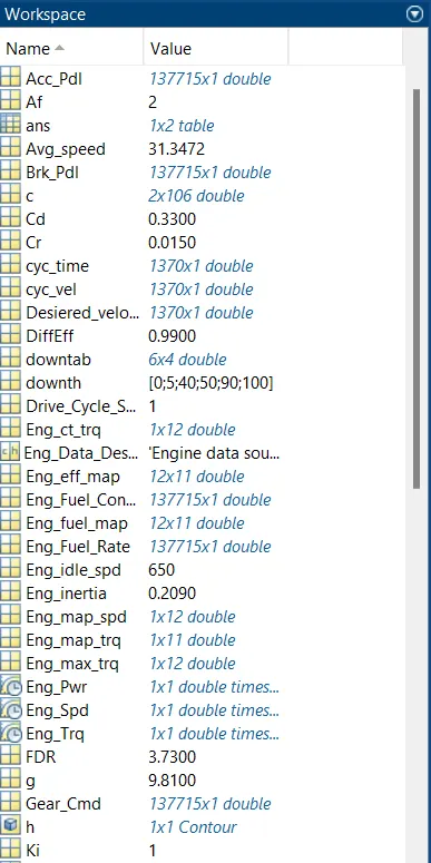
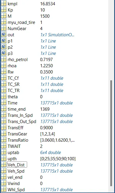
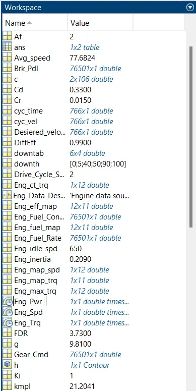
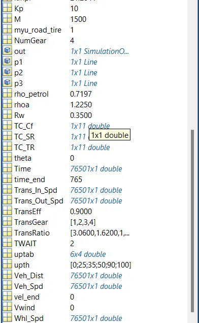
WORKSPACE

UDDS Drive Cycle

HWFET Drive Cycle

COMMAND WINDOW

UDDS Drive Cycle

HWFET Drive Cycle

RESULT

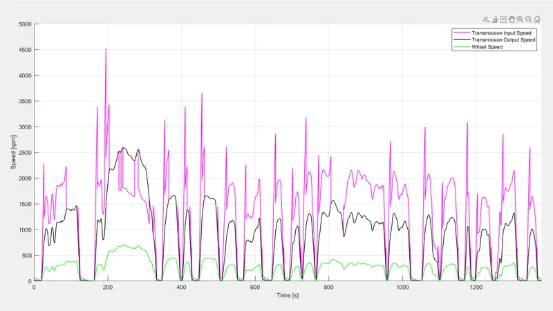
Time trace for engine, transmission input, transmission output and wheel speed : HWFET Drive Cycle

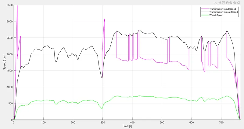
From both the graphs of UDDS & HWFET it is clearly visible that the up and down in torque input, torque output and the wheel speed is at high rate for UDDS cycle than the HWFET cycle.Also the transmission input and output torque seem to coinsides in the HWFT graph which may be due to there is no quick changes requied in the HWFET since it is a highway driving cycle.

b. Engine torque, engine power, fuel rate and fuel consumption: UDDS Drive Cycle

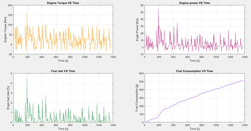
Engine torque, engine power, fuel rate and fuel consumption: HWFET Drive Cycle

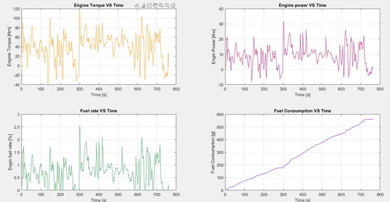
From comparision of both cycles graph it is again found that the torque requirement and the torque output is also bouncing at high rate for UDDS cycle but when comparing the fuel rate and fuel consumption graphs even though the bouncing is high in UDDS the fuel consumption is more in HWFET, this may be due to travelling in high speed constantly.Whereas in UDDS the speed is low.

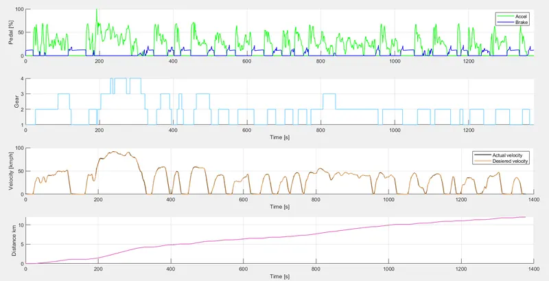
c. Accelerator and brake pedal, gear command, vehicle desired and actual speed, vehicle distance : UDDS Drive Cycle

Accelerator and brake pedal, gear command, vehicle desired and actual speed, vehicle distance : HWFET Drive Cycle

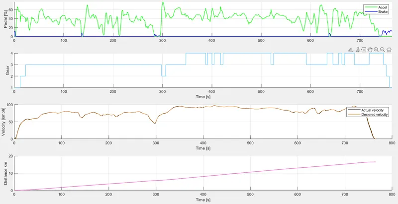
Here the acclerator peddel and brake peddel is applied frequently in UDDS cycle whereas in HWFET cylce the brake peddle is applied rarely.Also when we look in to the gear shifting In HWFET we can find the gear shift rarely where as in UDDS it is also done frequently.The actual velocity and desiered velocity in both the cases coincides.When we look into the distance graph in UDDS the covering of distance to not uniform whereas in HWFET the the graph is a uniformly increasing line.

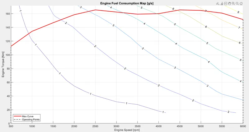
Engine operating points on engine fuel map : HWFET Drive Cycle

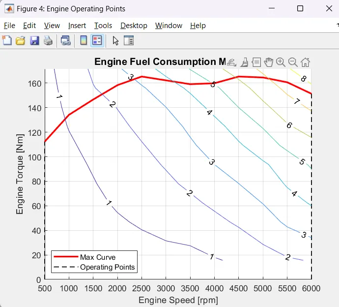
e. UDDS Drive Cycle

HWFET Drive Cycle

REFERENCE

• https://www.nyserda.ny.gov/All-Programs/Drive-Clean-Rebate-For-Electric-Cars-Program/About-Electric-Cars/Types-of-Cars#:~:text=Conventional%20vehicles%20use%20an%20internal,used%20to%20move%20the%20vehicle.
• https://www.researchgate.net/figure/Forward-facing-dynamic-vehicle-model_fig1_256202589