Project 1
Aim:- Analysis & Design raft foundation of a box culvert bridge having 12 M span and 5.5 M height in STAAD pro and applying loads as per IRC 6.
Que 1) Calculate the loads to be applied on the box as per IRC 6.
Given Data:-
- The span of structure = 12 M
- Height of structure = 5.5 M
- Safe bearing capacity of soil = 80 kN/m2
- Wearing coat fill on structure = 1.5 M
- Haunch size = 200 x 200 MM
- Soil density = 18 kN/m3
- Concrete M35
- Steel Fe500
Assumption and Design Data:-
Span in model = 12.7 M
Height of structure = 6.15 M
| No. of Cell | = | 1 | ||
| Clear Span (skew) | = | 12.00 | M |
| Clear Height at outer edge | = | 5.50 | M | |
| Clear Height at median edge | = | 5.50 | M |
| Width of Box | = | 12.50 | M | |
| Carriage Width | = | 11.50 | M | |
| Width of crash barrier | = | 0.50 | M |
| Width of Haunch | = | 0.20 | M | |
| Depth of Haunch | = | 0.20 | M |
| Depth of top slab | = | 0.60 | M | |
| Depth of bottom slab | = | 0.70 | M | |
| Depth of External Vertical wall | = | 0.70 | M |
| Safe Bearing capacity | = | 80.00 | KN/m2 | |
| Allowable Settlement | = | 75.00 | mm | |
| Spring Constanrt | = | 1066.67 | KN/m3 |
| Density of concrete | = | 25.00 | KN/m3 | |
| Bulk Density of soil | = | 18.00 | KN/m3 | |
| Density of submerge soil | = | 10.00 | KN/m3 | |
| Density of profile corrective course | = | 25.00 | KN/m3 | |
| Density of fill | = | 18.00 | KN/m3 | |
| Coefficient of earth pressure at rest | = | 0.50 |
| Maximum air shade temp. | = | 40.00 | 0/C | |
| Minimum air shade temp. | = | 12.50 | 0/C |
| Max Live Load on box for breaking force calculation | = | 700.00 | KN | |
| Design parameter | ||||
| Grade of Concrete | = | M | 35 | |
| Grade of Steel | = | Fe | 500 | |
| Clear cover for earth face structural component | = | 75 | mm | |
| Clear cover for inside face structural component | = | 50 | mm | |
| Clear Cover for foundation | = | 75 | mm | |
| Data for STAAD input | ||||
| No. of division of Bottom Slab | = | 10 |
Procedure Creating 2D STAAD model
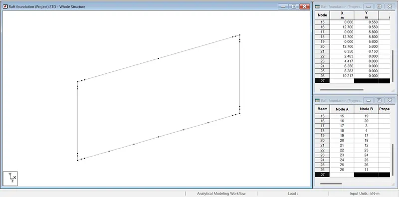
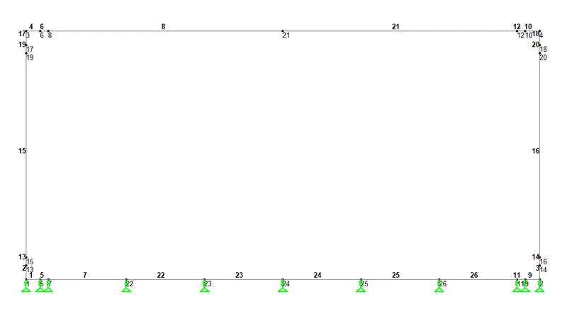
Creating a 2D model using a grid model with appropriate dimensions. For making a frame considering the centerline from both sides and assign proper distance nodes for haunches. after that we need to assign the properties to the structure with appropriate size. then we need to assign the support as fix but support then adding spring constant using calculation. spring constant calculated on the basis of safe bearing capicapity of soil.
Model Creating.
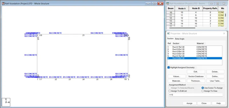
Assigning Material Properti.
Assigning Support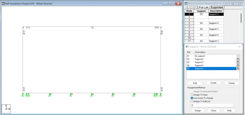
3D Model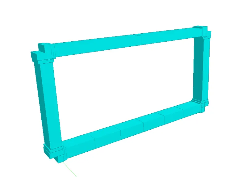
Assigning Loads on the model.
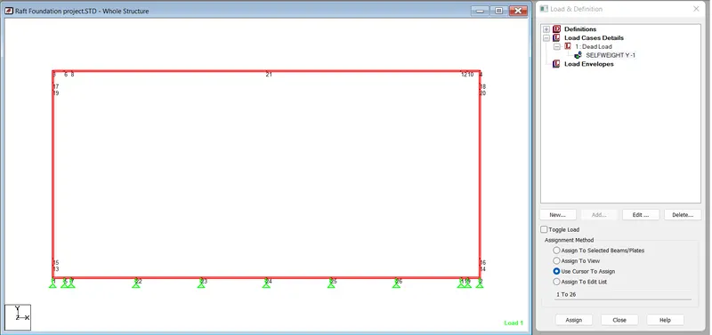
1. Dead Load
Step for assigning dead load.
Loading -> Load Case details -> Add -> Creat title as "Dead Load' -> Add -> stelect dead load and add again -> self weight -> Factor -1 -> Add -> Assign to view -> Assign.
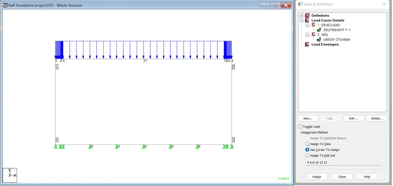
2. SIDL
| Super Imposed Dead Load | |||||
| Thickness of W.C + profile correction course | = | 1.5 | m | ||
| Load (UDL) on top slab | = | 37.5 | KN/m | ||
| Height of fill | = | 0 | m | ||
| Load (UDL) Load on top slab | = | 0 | KN/m | ||
| Total SIDL load on top slab | = | 37.5 | KN/m |
Step for assigning SIDL load n STADD.pro
Loading -> Load Case detail -> Add -> Create title as "SIDL" -> Add -> select SIDL and add again -> Member Load -> uniform force -> W1 37.5 direction as GY -> Add -> Select top member then select load -> Assign to selected beam -> assign.
3. Earth Pressure Load.
considering value,
At rest pressure is (Ka) 0.5
The density of soil is 18 kN/m3
| Earth pressure | |||||
| Thickness of top slab | = | 0.60 | m | ||
| Height of top hunch | = | 0.20 | m | ||
| Clear height between top & bottom slab | = | 5.50 | m | ||
| Height of bottom hunch | = | 0.20 | m | ||
| Thickness of bottom slab | = | 0.70 | m |
| Height from top (M) |
Intensity of Earth pressure (KN/m2) |
|||
| 1.40 | 1.40 | = | 12.60 | |
| 0.30 | 1.70 | = | 15.30 | |
| 0.20 | 1.90 | = | 17.10 | |
| 5.05 | 6.95 | = | 62.55 | |
| 0.20 | 7.15 | = | 64.35 | |
| 0.35 | 7.50 | = | 67.50 | |
Step for assigning load on model
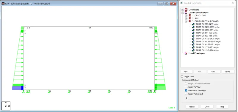
Loading > Load Case detail > Add > Create title as "Earth pressure" > Add > Select Earth Pressure load and add again > Member Load > Hyrdostatic > W1 = 67.50 and W2 = 12.60 diection as GX > Add > first select member then select load > Assign to selected beam > assign.
Repeat same procedure for all the member by changing the value of W1 and W2. in both the side
4. Live Load surcharge
Calculating Live Load surcharge.
Value assumption,
Coefficient of lateral earth pressure (K) is 0.5
Density of soil is (Y) 18 kN/m3
Equivalent height of soil for vehicular loading which shall be (h) 1.2 M.
`Delta`= k x y x h
| Live Load surcharge | |||||
| Uniform Intensity of loading | = | 10.8 | KN/m2 |
Below steps for assigning load on model.
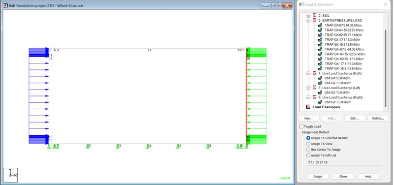
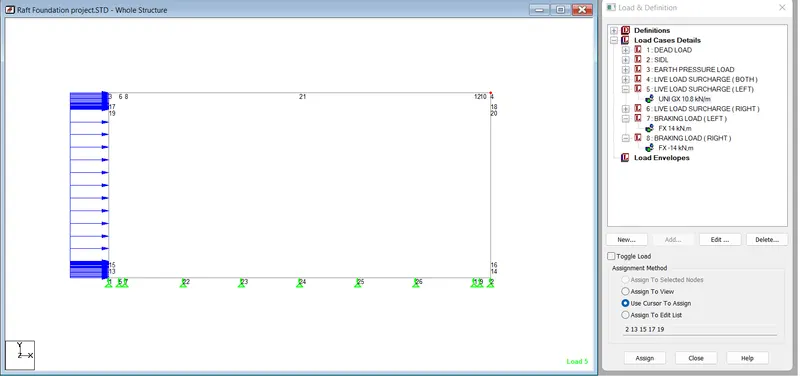
Loading -> Load Case detail -> Add -> Creat title as "Live Load surcharge" -> Add -> select Live Load surcharge and add again -> Member Load -> uniform force -> W1 10.8 direction as GX -> Add -> first select member then select load -> Assign to selected beam -> assign.
Repeating same procedure for different direction but value of W1 is -10.8.
Left Side
Right Side
5. Braking Forces.
Max Live Load on box ( for 2 lanes) is 700 kN/m2
Width of the box is 12.50 M
Total Braking force is 14 kN.
Below step for assigning braking force to STAAD model.
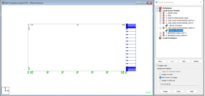
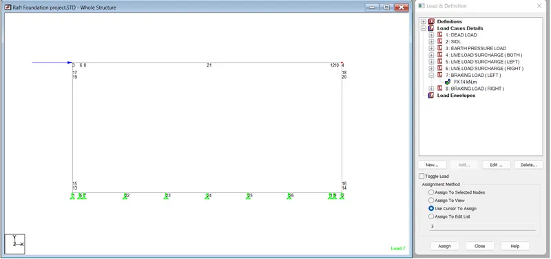
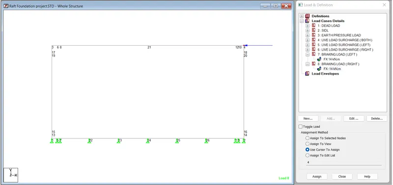
Loading -> Load Case detail -> Add -> Create title as "Braking Load" -> Add -> select Braking Load and add again -> Nodel load -> Fx = 14. -> add -> first select top node then select load -> Assign to selected node -> assign.
Repeat same procedure for different side whose node value of Fx is -14.
Left Side
Right Side
6. Temperature Load.
| 2.6 | Temperature | ||||
| Maximum effective bridge temp | = | 40.00 | C | ||
| Minimum effective bridge temp | = | 12.50 | C |
Effective Temperature Difference.
= (40 - 12.50)/2 + 10
= 13.75 + 10
- Temperature Rise is = 23.75.
Steps for assigning Load.
Loading -> Load Case detail -> Add -> Create title as "Temperature Load Rise" -> Add -> select Temperature Load (Rise) and add again -> Tempreature Load -> Temperatures -> Temp change elongation =23.75 -> Add -> first select member then select load -> Assign to selected beam -> assign.
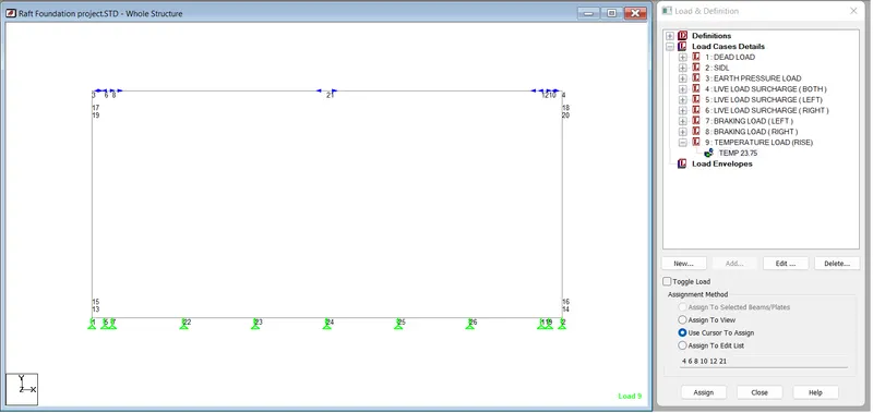
- Temperature Fall is = -23.75.
Steps for assigning Load.
Loading -> Load Case detail -> Add -> Creat title as "Temperature Load Fall" -> Add -> stelect Temperature Load (Fall) and add again -> Tempreature Load -> Temperatures -> Temp change elongation =-23.75 -> Add -> first select member then select load -> Assign to selected beam -> assign.
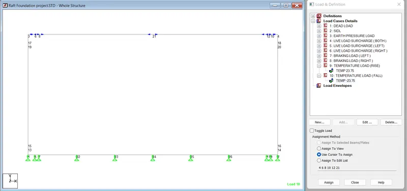
- Temperature Gradient (Rise)
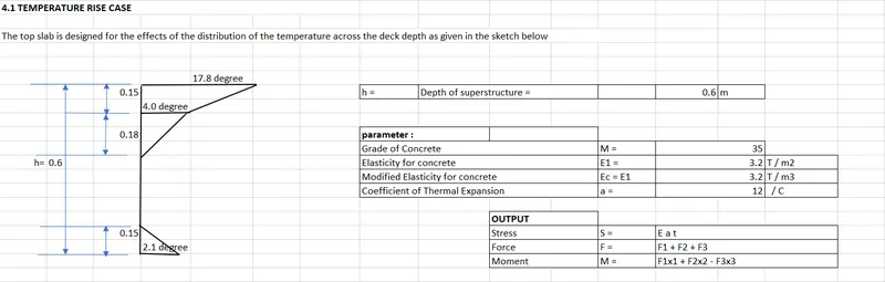
| TEMPERATURE RISE CASE | ||||||||||||
| Member Description | h | h1 | h2 | h3 | T1 | T2 | T3 | |||||
| (m) | (m) | (m) | (m) | / C | / C | / C | ||||||
| Top Slab | 0.6 | 0.15 | 0.18 | 0.15 | 17.8 | 4 | 2.1 | |||||
| Member Description | E a t S1 | S2 | S3 | F1 | F2 | F3 | F | |||||
| T / m2 | T / m2 | T / m2 | T | T | T | T | ||||||
| Top Slab | 683.52 | 153.60 | 80.64 | 56.96 | 12.80 | 6.72 | 76.48 | |||||
| Member Description | CG of Section fromTop | CG of Section From |
CG of TOP BLOCK from Top |
CG of MID BLOCK from Top |
CG of BOTTOM BLOCK from BOTTOM |
x1 | x2 | x3 | M | |||
| m | m | m | T-m | |||||||||
| Top Slab | 0.3 | 0.3 | 0.0601 | 0.21 | 0.05 | 0.2399 | 0.09 | 0.25 | 13.13717431 | |||
Steps for assigning Load.
Loading -> Load Case detail -> Add -> Create title as "Temperature Gradient (Rise)" -> Add -> select Temperature Gradient (Rise) and add again -> Nodal load -> Node -> Fx = 76.48 -> Add -> Mz = 13.14 -> (Again for other direction node) Fx = -76.48 & Mz - 13.14 -> Add -> select induidal node then select load -> Assign to selected node -> assign.
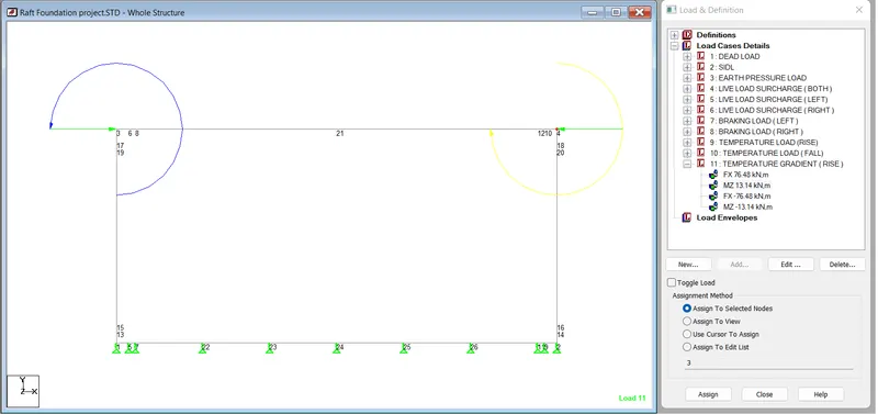
- Temperature Gradient (Fall)
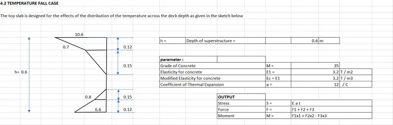
| TEMPERATURE RISE CASE | ||||||||||||||||
| Member Description | h | h1 | h2 | h3 | h4 | T1 | T2 | T3 | T4 | |||||||
| (m) | (m) | (m) | (m) | (m) | / C | / C | / C | / C | ||||||||
| Top Slab | 0.6 | 0.12 | 0.15 | 0.15 | 0.12 | 10.6 | 0.7 | 0.8 | 6.6 | |||||||
| Member Description | E a t S1 | S2 | S3 | S4 | F1 | F2 | F3 | F4 | F | |||||||
| T / m2 | T / m2 | T / m2 | T / m3 | T | T | T | T | T | ||||||||
| Top Slab | 407.04 | 26.88 | 30.72 | 253.44 | 26.04 | 2.02 | 2.30 | 17.0496 | 47.40 | |||||||
| Member Description | CG of Section fromTop | CG of Section From |
CG of TOP BLOCK from Top |
CG of MID BLOCK from Top |
CG of MID BLOCK from Bottom |
CG of BOTTOM BLOCK from BOTTOM |
x1 | x2 | x3 | x4 | M | |||||
| m | m | m | m | T-m | ||||||||||||
| Top Slab | 0.3 | 0.3 | 0.0395 | 0.17 | 0.17 | 0.05 | 0.2605 | 0.13 | 0.13 | 0.25 | 2.4822144 | |||||
Steps for assigning Load.
Loading -> Load Case detail -> Add -> CreatE title as "Temperature Gradient (Fall)" -> Add -> select Temperature Gradient (Fall) and add again -> Nodal load -> Node -> Fx = 47.40 -> Add -> Mz = 2.49 -> (Again for other direction node) Fx = -47.40 & Mz - 2.49 -> Add -> select induidal node then select load -> Assign to selected node -> assign.
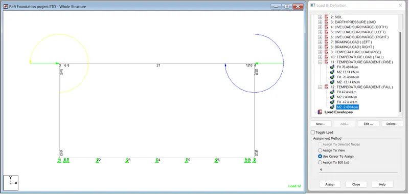
Analysis:
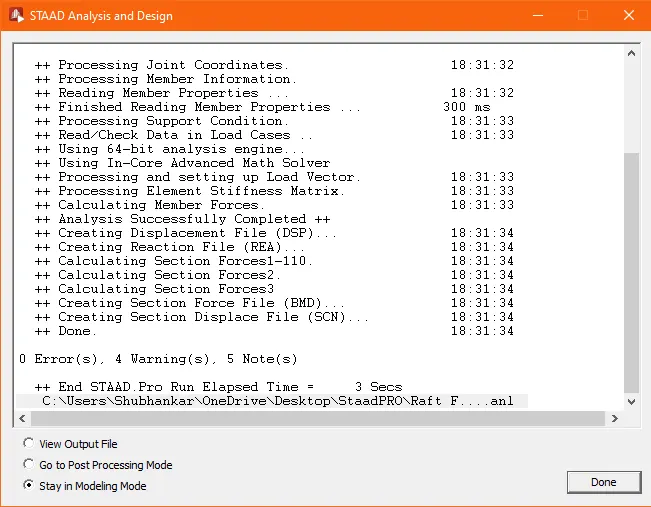
Analysis and Design > Click 'Define Commands' > Select "Perform Analysis" > Add > Click 'Run Analysis'
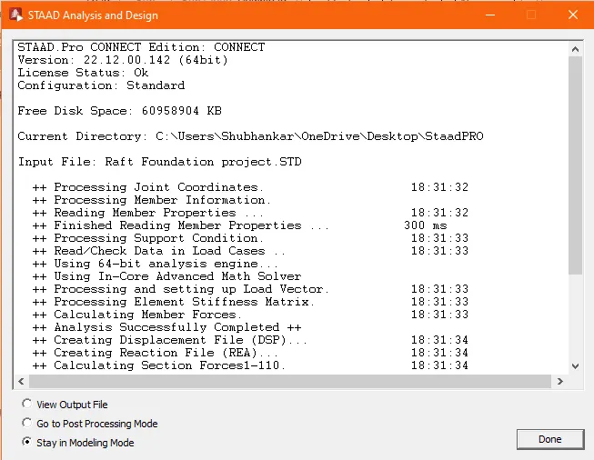
Zero Errors found:
Que 2) Live load analysis and effective width calculation for 70 R and Class A to be done.
For the 70 R &b Class A loading we have to make another new model in STADD.Pro, for making model repeating same procedure as mention above size and properties also same.
Calculating Load of Class 70 R vehical loading.
| One no of 70 R tracked | |||
| Carriageway Live Load | = | 700 | KN |
| Transverse eccentr of live load | = | 3.1 | m |
| Transverse Movement | = | 2170 | KNm |
| UDL due to ecc. Of CWLL | = | 7.31 | KN/m |
| Longitudinal eccentr of live load | = | 2.215 | m |
| Longitudinal Movement | = | 1550.5 | KNm |
| UDL due to ecc. Of CWLL | = | 5.73 | KN/m |
| Two no of 70 R tracked | |||
| Carriageway Live Load | = | 1400 | KN |
| Transverse eccentr of live load | = | 0.35 | m |
| Transverse Movement | = | 490 | KNm |
| UDL due to ecc. Of CWLL | = | 1.65 | KN/m |
| Longitudinal eccentr of live load | = | 2.215 | m |
| Longitudinal Movement | = | 3101 | |
| UDL due to ecc. Of CWLL | = | 11.45 |
| 1 | Design Data | |||
| No. of Cell | = | 1 | ||
| Clear Span (skew) | = | 12.00 | m | |
| Clear Height at outer edge | = | 5.50 | m | |
| Width of Box | = | 12.50 | m | |
| Carriage Width | = | 11.50 | m | |
| Width of crash barrier | = | 0.50 | m | |
| Width of footpath / safty kerd | = | 0.00 | m | |
| Width of Haunch | = | 0.20 | m | |
| Depth of Haunch | = | 0.20 | m | |
| Thickness of waring coat | = | 1.50 | m | |
| Thickness of fill over top slab excluding wearing coat | = | 0.00 | m | |
| Depth of top slab | = | 0.60 | m | |
| Depth of bottom slab | = | 0.70 | m | |
| Depth of External Vertial wall | = | 0.70 | m |
| For 70 R - Tracked | ||||
| Clear distance | = | 1.2 | m | |
| Width of track (transverse to traffic direction) | = | 0.84 | m | |
| Width of track (along traffic direction) | = | 4.57 | m | |
| Total width of vehical | = | 2.9 | m | |
| Width center to center of wheel | = | 2.06 | m |
| For 70 R - Tracked | ||||
| Impact factor | ||||
| Impact factor = | 10.0 | % | 1.10 | |
| Effective Dispersion Width | ||||
| Dispersion of loads through fills and wearing coat ( at 45degree angle) | ||||
| b = tyre width along traffic flow | = | 4.57 | m | |
| wc = wearing coat | = | 1.50 | m | |
| d = effective depth of slab | = | 0.60 | m | |
| s = thickness of soil above box | = | 0.00 | m | |
| Hence, dispersion width | = | 8.77 | m | |
| Calculation of effective width | ||||
| k = constant depending on b/lo | = | 2.335 | ||
| lo = effective span | = | 12.7 | m | |
| x = Distance of center fo gravity from nearest support | = | 6.35 | m | |
| x = Distance of center fo gravity from nearest support | = | 2.285 | m | |
| b = tyre width across traffic flow | = | 0.84 | m | |
| wc = wearing coat | = | 0 | m | |
| bt = width of tyre + 2 x thickness of w.c | = | 3.84 | m | |
| Hence, beff for max movement case | = | 6.508 | m | |
| Hence, beff for max vertical load case | = | 8.77 | m | |
| For 70 R - Tracked | = | 770 | KN | |
| Pressureon top slab : | ||||
| (i) Maximum movement case : | ||||
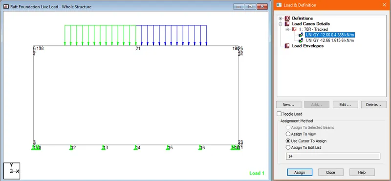
| UDL due to live load | = | 12.66 | KN/m2 | |
| dispersion length of live load in longitudinal direction | = | 8.77 | m | |
| transverse dispersion | = | 6.93 | m | |
| (ii) Maximum vertical load on wall : | ||||
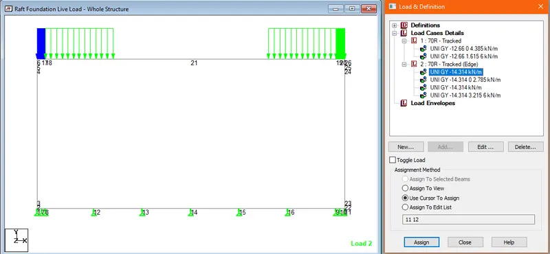
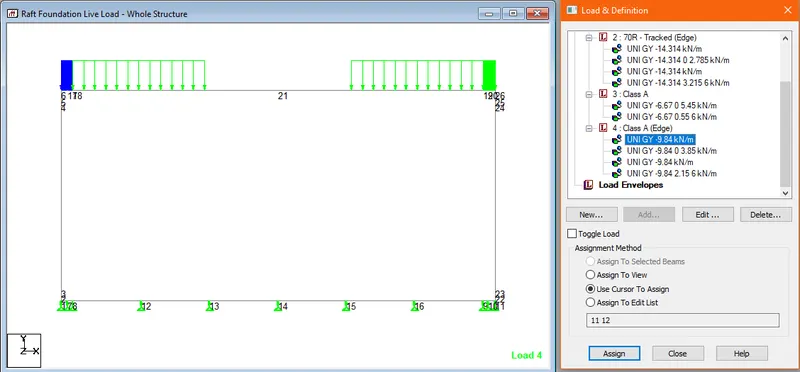
| UDL due to live load | = | 14.314 | KN/m2 | |
| dispersion length of live load in longitudinal direction | = | 6.67 | m | |
| transverse dispersion | = | 8.07 | m | |
Steps for assigning Load.
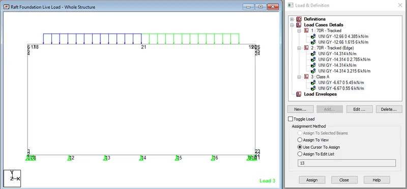
Loading -> Load Case detail -> Add -> Create title as "70 R Tracked" -> Add -> select 70 R Tracked and add again -> member load -> Uniform force -> W1= -12.66 & d1 = 0, d2 = 4.385 -> first select member then select load -> Assign to selected beam -> assign.
Repeat Same procedure for other member with d1 = 1.615, d2 = 6.
- Maximum moment case
- Maximum vertical load on wall
| For Class - A | ||||
| Clear distance | = | 0.150 | m | |
| Width of track (transverse to traffic direction) | = | 0.500 | m | |
| Width of track (along traffic direction) | = | 4.397 | m | |
| Total width of vehical | = | 1.800 | m | |
| Width center to center of wheel | = | 1.300 | m |
| For Class - A Loading | ||||
| Impact factor | ||||
| Impact factore = | 20 | % | 1.20 | |
| Effective Dispersion Width | ||||
| Dispersion of loads through fills and wearing coat ( at 45degree angle) | ||||
| b = tyre width along traffic flow | = | 4.397 | m | |
| wc = wearing coat | = | 1.5 | m | |
| d = effective depth of slab | = | 0.60 | m | |
| s = thickness of soil above box | = | 0.00 | m | |
| Hence, dispersion width | = | 8.597 | m | |
| Calculation of effective width | ||||
| k = constant depending on b/lo | = | 2.335 | ||
| lo = effective span | = | 12.5 | m | |
| x = Distance of center fo gravity from nearest support | = | 5.1 | m | |
| x = Distance of center fo gravity from nearest support | = | 2.199 | m | |
| b = tyre width across traffic flow | = | 0.5 | m | |
| wc = wearing coat | = | 0 | m | |
| bt = width of tyre + 2 x thickness of w.c | = | 3.5 | m | |
| Hence, beff for max movement case | = | 13.31 | m | |
| Hence, beff for max vertical load case | = | 8.597 | m | |
| For Class A Loading | 554 | KN | ||
| Pressureon top slab : | ||||
| (i) Maximum movement case : | ||||
| Class- A loading is disperseed with overlapping in both the direction | ||||
| UDL due to live load | = | 6.67 | KN/m2 | |
| Longitudinal dispersion | = | 10.90 | m | |
| transverse dispersion | = | 9.15 | m | |
| (ii) Maximum vertical load on wall : | ||||
| UDL due to live load | = | 9.84 | KN/m2 | |
| dispersion length of live load in longitudinal direction | = | 8.80 | m | |
| transverse dispersion | = | 7.68 | m | |
Steps for assigning load on structure is same as mention above.
- Maximum movement case
- Maximum vertical load on wall
Analysis:
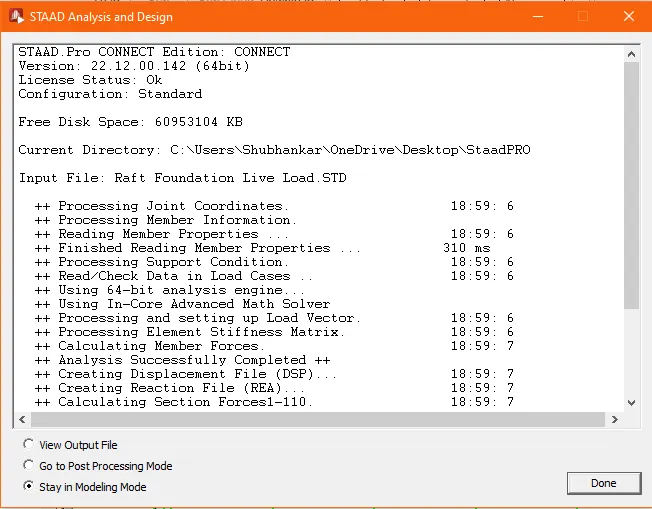
Analysis and Design > Click 'Define Commands' > Select "Perform Analysis" > Add > Click 'Run Analysis'
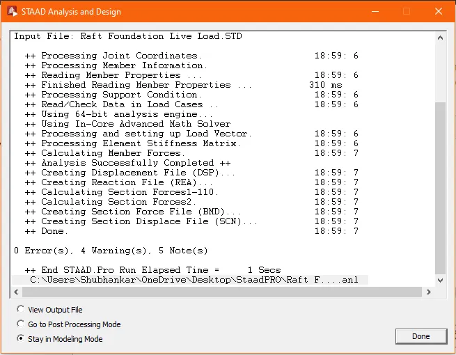
Zero Errors found:
Result
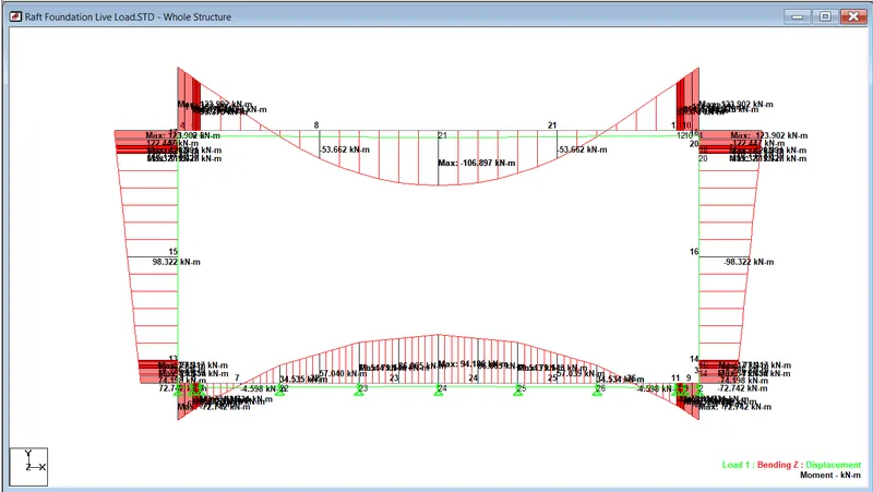
- Maximum Movemet Case of Vehical Load Case
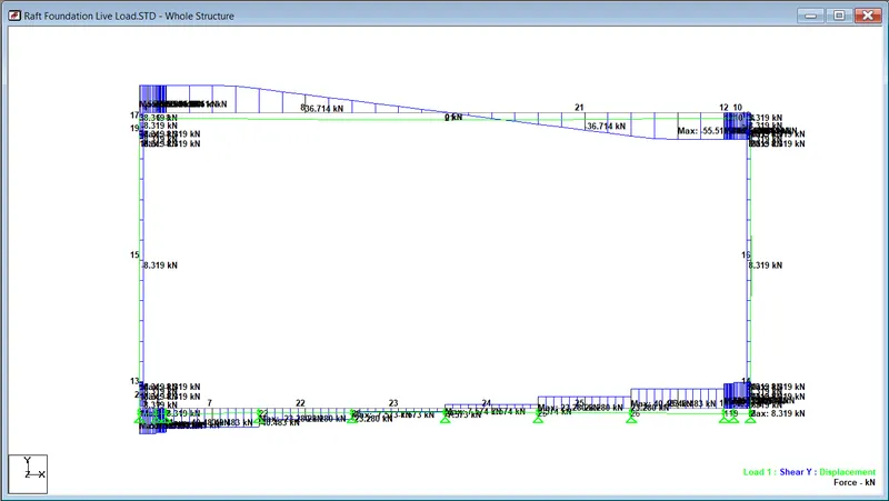
- Maximum Shear Case of Vehical Live Load
Que 3) Make Load combinations as per IRC 6 for ULS, SLS rare and quasi
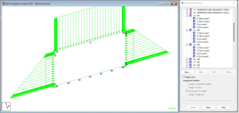
Making combination for finding maximum bending movement case and shear force case of each member.
Combination For Ultimate Limit State case.
| Dead Load ,SIDL , Earth Pressure, Live Load Surcharge ( Accompanying) | |||||||
| 1 | DL | + | SIDL | + | EP Load | + | LL - S (Both Side) |
| 1.35 | 1.35 | 1 | 1.2 | ||||
| 2 | DL | + | SIDL | + | EP Load | + | LL - S (Lefth Side) |
| 1.35 | 1.35 | 1 | 1.2 | ||||
| 3 | DL | + | SIDL | + | EP Load | + | LL - S (Right Side) |
| 1.35 | 1.35 | 1 | 1.2 | ||||
| Dead Load ,SIDL , Earth Pressure, Live Load Surcharge, Temp Rise ( Accompanying) | |||||||||
| 1 | DL | + | SIDL | + | EP Load | + | LL - S (Both Side) | + | Temp Rise |
| 1.35 | 1.35 | 1 | 1.2 | 0.9 | |||||
| 2 | DL | + | SIDL | + | EP Load | + | LL - S (Lefth Side) | + | Temp Rise |
| 1.35 | 1.35 | 1 | 1.2 | 0.9 | |||||
| 3 | DL | + | SIDL | + | EP Load | + | LL - S (Right Side) | + | Temp Rise |
| 1.35 | 1.35 | 1 | 1.2 | 0.9 | |||||
| Dead Load ,SIDL , Earth Pressure, Live Load Surcharge, Temp Fall ( Accompanying) | |||||||||
| 1 | DL | + | SIDL | + | EP Load | + | LL - S (Both Side) | + | Temp Fall |
| 1.35 | 1.35 | 1 | 1.2 | 0.9 | |||||
| 2 | DL | + | SIDL | + | EP Load | + | LL - S (Lefth Side) | + | Temp Fall |
| 1.35 | 1.35 | 1 | 1.2 | 0.9 | |||||
| 3 | DL | + | SIDL | + | EP Load | + | LL - S (Right Side) | + | Temp Fall |
| 1.35 | 1.35 | 1 | 1.2 | 0.9 | |||||
| Dead Load ,SIDL , Earth Pressure, Live Load Surcharge, Temp Gradient Rise ( Accompanying) | |||||||||
| 1 | DL | + | SIDL | + | EP Load | + | LL - S (Both Side) | + | Temp Gradient Rise |
| 1.35 | 1.35 | 1 | 1.2 | 0.9 | |||||
| 2 | DL | + | SIDL | + | EP Load | + | LL - S (Lefth Side) | + | Temp Gradient Rise |
| 1.35 | 1.35 | 1 | 1.2 | 0.9 | |||||
| 3 | DL | + | SIDL | + | EP Load | + | LL - S (Right Side) | + | Temp Gradient Rise |
| 1.35 | 1.35 | 1 | 1.2 | 0.9 | |||||
| Dead Load ,SIDL , Earth Pressure, Live Load Surcharge, Temp Gradient Fall ( Accompanying) | |||||||||
| 1 | DL | + | SIDL | + | EP Load | + | LL - S (Both Side) | + | Temp Gradient Fall |
| 1.35 | 1.35 | 1 | 1.2 | 0.9 | |||||
| 2 | DL | + | SIDL | + | EP Load | + | LL - S (Lefth Side) | + | Temp Gradient Fall |
| 1.35 | 1.35 | 1 | 1.2 | 0.9 | |||||
| 3 | DL | + | SIDL | + | EP Load | + | LL - S (Right Side) | + | Temp Gradient Fall |
| 1.35 | 1.35 | 1 | 1.2 | 0.9 | |||||
| Dead Load (Relieving) ,SIDL , Earth Pressure ( Leading) , Live Load Surcharge | |||||||
| 1 | DL | + | SIDL | + | EP Load | + | LL - S (Both Side) |
| 1 | 1 | 1.5 | 1.2 | ||||
| 2 | DL | + | SIDL | + | EP Load | + | LL - S (Lefth Side) |
| 1 | 1 | 1.5 | 1.2 | ||||
| 3 | DL | + | SIDL | + | EP Load | + | LL - S (Right Side) |
| 1 | 1 | 1.5 | 1.2 | ||||
| Dead Load (Relieving) ,SIDL , Earth Pressure ( Leading), Live Load Surcharge, Temp Rise ( Accompanying) | |||||||||
| 1 | DL | + | SIDL | + | EP Load | + | LL - S (Both Side) | + | Temp Rise |
| 1 | 1 | 1.5 | 1.2 | 0.9 | |||||
| 2 | DL | + | SIDL | + | EP Load | + | LL - S (Lefth Side) | + | Temp Rise |
| 1 | 1 | 1.5 | 1.2 | 0.9 | |||||
| 3 | DL | + | SIDL | + | EP Load | + | LL - S (Right Side) | + | Temp Rise |
| 1 | 1 | 1.5 | 1.2 | 0.9 | |||||
| Dead Load (Relieving) ,SIDL , Earth Pressure ( Leading), Live Load Surcharge, Temp Fall ( Accompanying) | |||||||||
| 1 | DL | + | SIDL | + | EP Load | + | LL - S (Both Side) | + | Temp Fall |
| 1 | 1 | 1.5 | 1.2 | 0.9 | |||||
| 2 | DL | + | SIDL | + | EP Load | + | LL - S (Lefth Side) | + | Temp Fall |
| 1 | 1 | 1.5 | 1.2 | 0.9 | |||||
| 3 | DL | + | SIDL | + | EP Load | + | LL - S (Right Side) | + | Temp Fall |
| 1 | 1 | 1.5 | 1.2 | 0.9 | |||||
| Dead Load (Relieving) ,SIDL , Earth Pressure ( Leading) , Live Load Surcharge, Temp Gredient (Rise) | |||||||||
| 1 | DL | + | SIDL | + | EP Load | + | LL - S (Both Side) | + | Temp Gradient Rise |
| 1 | 1 | 1.5 | 1.2 | 0.9 | |||||
| 2 | DL | + | SIDL | + | EP Load | + | LL - S (Lefth Side) | + | Temp Gradient Rise |
| 1 | 1 | 1.5 | 1.2 | 0.9 | |||||
| 3 | DL | + | SIDL | + | EP Load | + | LL - S (Right Side) | + | Temp Gradient Rise |
| 1 | 1 | 1.5 | 1.2 | 0.9 | |||||
| Dead Load (Relieving) ,SIDL , Earth Pressure ( Leading) , Live Load Surcharge, Temp Gredient (Fall) | |||||||||
| 1 | DL | + | SIDL | + | EP Load | + | LL - S (Both Side) | + | Temp Gredient (Fall) |
| 1 | 1 | 1.5 | 1.2 | 0.9 | |||||
| 2 | DL | + | SIDL | + | EP Load | + | LL - S (Lefth Side) | + | Temp Gredient (Fall) |
| 1 | 1 | 1.5 | 1.2 | 0.9 | |||||
| 3 | DL | + | SIDL | + | EP Load | + | LL - S (Right Side) | + | Temp Gredient (Fall) |
| 1 | 1 | 1.5 | 1.2 | 0.9 | |||||
| Dead Load (Relieving) ,SIDL , Earth Pressure ( Accomplying) , Live Load Surcharge, Temp Rise (Leading) | |||||||||
| 1 | DL | + | SIDL | + | EP Load | + | LL - S (Both Side) | + | Temp Fall |
| 1 | 1 | 1 | 1.2 | 1.5 | |||||
| 2 | DL | + | SIDL | + | EP Load | + | LL - S (Lefth Side) | + | Temp Fall |
| 1 | 1 | 1 | 1.2 | 1.5 | |||||
| 3 | DL | + | SIDL | + | EP Load | + | LL - S (Right Side) | + | Temp Fall |
| 1 | 1 | 1 | 1.2 | 1.5 | |||||
Results.
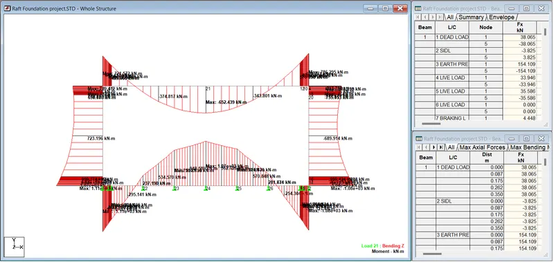
- Maximum Movemet Case for ULS combination.
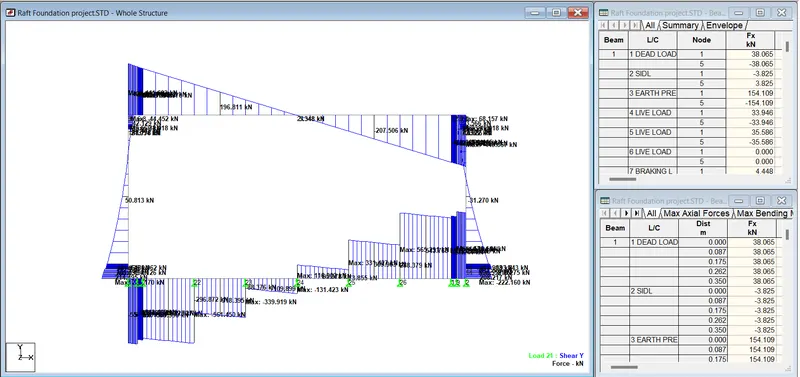
- Maximum Shear Case for ULS Combination.
| FORCE SUMMARY (ULS) | |||||||||
| 5.1 Ultimate Limit State (ULS) | |||||||||
| LL model | ULS model | ||||||||
| Live Load case (unfactored) from STAAD output |
Normal Load case (factored) from STAAD output |
Normal Load Case + Live Load |
Design Values | ||||||
| Movement (kN-m) |
Shear at D dist KN |
Movement (kN-m) |
Shear at D dist KN |
Movement (kN-m) |
Shear at D dist KN |
Movement (kN-m) |
Shear at D dist KN |
||
| 21 | Mid top | 0 | |||||||
| Mid bot | 106.897 | 652 | 758.897 | 758.897 | |||||
| 4 & 6 | Support top | 123.904 | 721 | 445.893 | 844.904 | 445.893 | 844.904 | 445.893 | |
| Support bot | 0 | ||||||||
| 17 & 19 | Outside | 123.904 | 719.442 | 156.57 | 843.346 | 156.57 | 843.346 | 156.57 | |
| Inside | 0 | ||||||||
| 15 | Outside | 98.322 | 723.196 | 821.518 | 821.518 | ||||
| Inside | 0 | ||||||||
| 13 & 2 | Outside | 77.13 | 829.35 | 276.456 | 906.48 | 276.456 | 906.48 | 276.456 | |
| Inside | 0 | ||||||||
| 1 & 5 | Support top | 57.04 | 842.62 | 428.307 | 899.66 | 428.307 | 899.66 | 428.307 | |
| Support bot | 72.74 | 678.313 | 751.053 | ||||||
| 7 , 22 & 23 | top | 79.54 | 759.799 | 839.339 | 839.339 | ||||
| bottom | 0 | ||||||||
Combination For Ultimate Serviceability Limit State ( Rare Combination)
| Dead Load ,SIDL , Earth Pressure ( Leading) , Live Load Surcharge | |||||||
| 1 | DL | + | SIDL | + | EP Load | + | LL - S (Both Side) |
| 1 | 1 | 1 | 0.8 | ||||
| 2 | DL | + | SIDL | + | EP Load | + | LL - S (Lefth Side) |
| 1 | 1 | 1 | 0.8 | ||||
| 3 | DL | + | SIDL | + | EP Load | + | LL - S (Right Side) |
| 1 | 1 | 1 | 0.8 | ||||
| Dead Load ,SIDL , Earth Pressure , Live Load Surcharge, Temp Rise (Accompanying) | |||||||||
| 1 | DL | + | SIDL | + | EP Load | + | LL - S (Both Side) | + | Temp Rise (Accompanying) |
| 1 | 1 | 1 | 0.8 | 0.6 | |||||
| 2 | DL | + | SIDL | + | EP Load | + | LL - S (Lefth Side) | + | Temp Rise (Accompanying) |
| 1 | 1 | 1 | 0.8 | 0.6 | |||||
| 3 | DL | + | SIDL | + | EP Load | + | LL - S (Right Side) | + | Temp Rise (Accompanying) |
| 1 | 1 | 1 | 0.8 | 0.6 | |||||
| Dead Load ,SIDL , Earth Pressure , Live Load Surcharge, Temp Fall (Acompanying) | |||||||||
| 1 | DL | + | SIDL | + | EP Load | + | LL - S (Both Side) | + | Temp Fall |
| 1 | 1 | 1 | 0.8 | 0.6 | |||||
| 2 | DL | + | SIDL | + | EP Load | + | LL - S (Lefth Side) | + | Temp Fall |
| 1 | 1 | 1 | 0.8 | 0.6 | |||||
| 3 | DL | + | SIDL | + | EP Load | + | LL - S (Right Side) | + | Temp Fall |
| 1 | 1 | 1 | 0.8 | 0.6 | |||||
| Dead Load ,SIDL , Earth Pressure , Live Load Surcharge, Temp Gradient Rise (Accompanying) | |||||||||
| 1 | DL | + | SIDL | + | EP Load | + | LL - S (Both Side) | + | Temp Gradient Rise (Accompanying) |
| 1 | 1 | 1 | 0.8 | 0.6 | |||||
| 2 | DL | + | SIDL | + | EP Load | + | LL - S (Lefth Side) | + | Temp Gradient Rise (Accompanying) |
| 1 | 1 | 1 | 0.8 | 0.6 | |||||
| 3 | DL | + | SIDL | + | EP Load | + | LL - S (Right Side) | + | Temp Gradient Rise (Accompanying) |
| 1 | 1 | 1 | 0.8 | 0.6 | |||||
| Dead Load ,SIDL , Earth Pressure , Live Load Surcharge, Temp Gradient Fall (Accompanying) | |||||||||
| 1 | DL | + | SIDL | + | EP Load | + | LL - S (Both Side) | + | Temp Gradient Fall (Accompanying) |
| 1 | 1 | 1 | 0.8 | 0.6 | |||||
| 2 | DL | + | SIDL | + | EP Load | + | LL - S (Lefth Side) | + | Temp Gradient Fall (Accompanying) |
| 1 | 1 | 1 | 0.8 | 0.6 | |||||
| 3 | DL | + | SIDL | + | EP Load | + | LL - S (Right Side) | + | Temp Gradient Fall (Accompanying) |
| 1 | 1 | 1 | 0.8 | 0.6 | |||||
| Dead Load ,SIDL , Earth Pressure , Live Load Surcharge, Temp Rise (Leading) | |||||||||
| 1 | DL | + | SIDL | + | EP Load | + | LL - S (Both Side) | + | Temp Rise (Leading) |
| 1 | 1 | 1 | 0.8 | 1 | |||||
| 2 | DL | + | SIDL | + | EP Load | + | LL - S (Lefth Side) | + | Temp Rise (Leading) |
| 1 | 1 | 1 | 0.8 | 1 | |||||
| 3 | DL | + | SIDL | + | EP Load | + | LL - S (Right Side) | + | Temp Rise (Leading) |
| 1 | 1 | 1 | 0.8 | 1 | |||||
| Dead Load ,SIDL , Earth Pressure , Live Load Surcharge, Temp Fall (Leading) | |||||||||
| 1 | DL | + | SIDL | + | EP Load | + | LL - S (Both Side) | + | Temp Fall (Leading) |
| 1 | 1 | 1 | 0.8 | 1 | |||||
| 2 | DL | + | SIDL | + | EP Load | + | LL - S (Lefth Side) | + | Temp Fall (Leading) |
| 1 | 1 | 1 | 0.8 | 1 | |||||
| 3 | DL | + | SIDL | + | EP Load | + | LL - S (Right Side) | + | Temp Fall (Leading) |
| 1 | 1 | 1 | 0.8 | 1 | |||||
| Dead Load ,SIDL , Earth Pressure , Live Load Surcharge, Temp Gradient Rise (Leading) | |||||||||
| 1 | DL | + | SIDL | + | EP Load | + | LL - S (Both Side) | + | Temp Gradient Rise (Leading) |
| 1 | 1 | 1 | 0.8 | 1 | |||||
| 2 | DL | + | SIDL | + | EP Load | + | LL - S (Lefth Side) | + | Temp Gradient Rise (Leading) |
| 1 | 1 | 1 | 0.8 | 1 | |||||
| 3 | DL | + | SIDL | + | EP Load | + | LL - S (Right Side) | + | Temp Gradient Rise (Leading) |
| 1 | 1 | 1 | 0.8 | 1 | |||||
| Dead Load ,SIDL , Earth Pressure , Live Load Surcharge, Temp Gradient Fall (Leading) | |||||||||
| 1 | DL | + | SIDL | + | EP Load | + | LL - S (Both Side) | + | Temp Gradient Fall (Leading) |
| 1 | 1 | 1 | 0.8 | 1 | |||||
| 2 | DL | + | SIDL | + | EP Load | + | LL - S (Lefth Side) | + | Temp Gradient Fall (Leading) |
| 1 | 1 | 1 | 0.8 | 1 | |||||
| 3 | DL | + | SIDL | + | EP Load | + | LL - S (Right Side) | + | Temp Gradient Fall (Leading) |
| 1 | 1 | 1 | 0.8 | 1 | |||||
Result Maximum Case.
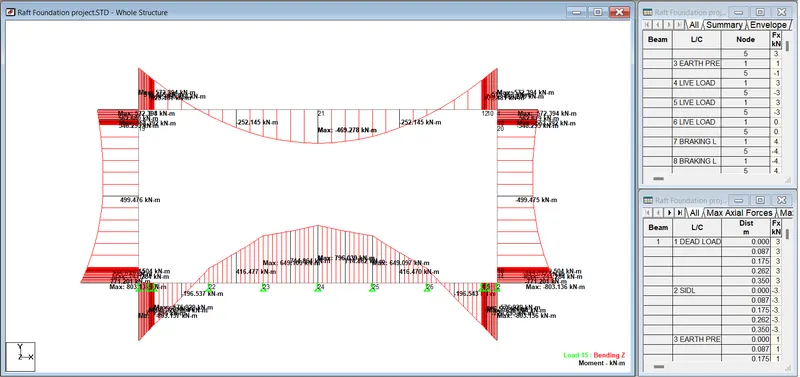
Normal Load Case.
Normal Load Case + Temp (Accompanying).
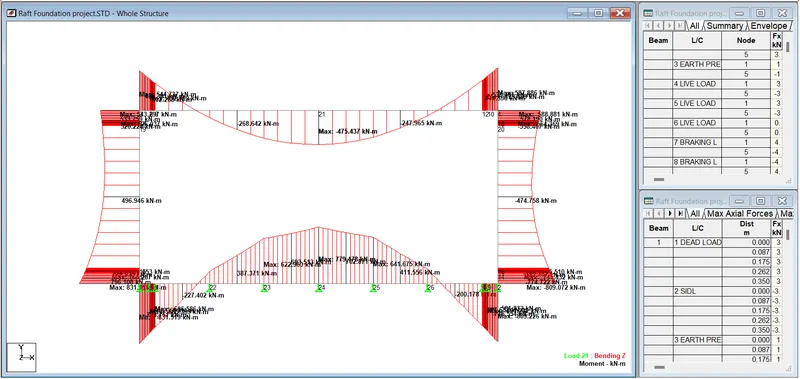
Normal Load Case + Temp (Leading).
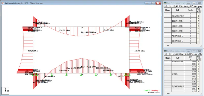
| FORCE SUMMARY (SLS) | |||||||||
| 5.2 Servicebility Limit State | |||||||||
| 5.2.1 Rare Combination | LL model | SLS (rare) | model | SLS (rare) | model | SLS (rare) | model | ||
| Live Load case (unfactored) from STAAD output |
Normal Load case (factored) from STAAD output |
Normal Load Case + Live Load |
Normal Load Case With Temperature Load (Accomp) |
Normal Load Case With Temperature + Live Load (Accomp) |
Normal Load Case With Temperature Load (Leading) |
Normal Load Case With Temperature + Live Load (Leading) |
Design Value |
||
| Moment kN-N | Moment kN-N | Moment kN-N | Moment kN-N | Moment kN-N | Moment kN-N | Moment kN-N | Moment kN-N | ||
| 21 | Mid top | 0 | |||||||
| Mid bot | 106.897 | 469.278 | 576.175 | 475.437 | 582.334 | 481.501 | 588.398 | 588.398 | |
| 4 & 6 | Support top | 123.904 | 572.364 | 696.268 | 544.737 | 668.641 | 538.673 | 662.577 | 696.268 |
| Support bot | 0 | ||||||||
| 17 & 19 | Outside | 123.904 | 572.395 | 696.299 | 543.297 | 667.201 | 537.233 | 661.137 | 696.299 |
| Inside | 0 | ||||||||
| 15 | Outside | 98.322 | 500 | 598.322 | 496.946 | 595.268 | 498.276 | 596.598 | 598.322 |
| Inside | 0 | ||||||||
| 13 & 2 | Outside | 77.13 | 803.137 | 880.267 | 831.058 | 908.188 | 839.782 | 916.912 | 916.912 |
| Inside | 0 | 0 | |||||||
| 1 & 5 | Support top | 57.04 | 715 | 772.04 | 622.1 | 679.14 | 614.784 | 671.824 | 772.04 |
| Support bot | 72.74 | 803.137 | 875.877 | 831.519 | 904.259 | 840.234 | 912.974 | 912.974 | |
| 7 , 22 & 23 | top | 79.54 | 769 | 848.54 | 779.478 | 859.018 | 771.439 | 850.979 | 859.018 |
| bottom | 0 | ||||||||
Combination For Ultimate Serviceability Limit State ( Quasi Combination)
| Dead Load ,SIDL , Earth Pressure ( Leading) , Live Load Surcharge | |||||||
| 1 | DL | + | SIDL | + | EP Load | + | LL - S (Both Side) |
| 1 | 1 | 1 | 0 | ||||
| 2 | DL | + | SIDL | + | EP Load | + | LL - S (Lefth Side) |
| 1 | 1 | 1 | 0 | ||||
| 3 | DL | + | SIDL | + | EP Load | + | LL - S (Right Side) |
| 1 | 1 | 1 | 0 | ||||
| Dead Load ,SIDL , Earth Pressure , Live Load Surcharge, Temp Rise (Accompanying) | |||||||||
| 1 | DL | + | SIDL | + | EP Load | + | LL - S (Both Side) | + | Temp Rise (Accompanying) |
| 1 | 1 | 1 | 0 | 0.5 | |||||
| 2 | DL | + | SIDL | + | EP Load | + | LL - S (Lefth Side) | + | Temp Rise (Accompanying) |
| 1 | 1 | 1 | 0 | 0.5 | |||||
| 3 | DL | + | SIDL | + | EP Load | + | LL - S (Right Side) | + | Temp Rise (Accompanying) |
| 1 | 1 | 1 | 0 | 0.5 | |||||
| Dead Load ,SIDL , Earth Pressure , Live Load Surcharge, Temp Fall (Accompanying) | |||||||||
| 1 | DL | + | SIDL | + | EP Load | + | LL - S (Both Side) | + | Temp Fall (Accompanying) |
| 1 | 1 | 1 | 0 | 0.5 | |||||
| 2 | DL | + | SIDL | + | EP Load | + | LL - S (Lefth Side) | + | Temp Fall (Accompanying) |
| 1 | 1 | 1 | 0 | 0.5 | |||||
| 3 | DL | + | SIDL | + | EP Load | + | LL - S (Right Side) | + | Temp Fall (Accompanying) |
| 1 | 1 | 1 | 0 | 0.5 | |||||
| Dead Load ,SIDL , Earth Pressure , Live Load Surcharge, Temp Gradient Rise (Accompanying) | |||||||||
| 1 | DL | + | SIDL | + | EP Load | + | LL - S (Both Side) | + | Temp Gradient Rise (Accompanying) |
| 1 | 1 | 1 | 0 | 0.5 | |||||
| 2 | DL | + | SIDL | + | EP Load | + | LL - S (Lefth Side) | + | Temp Gradient Rise (Accompanying) |
| 1 | 1 | 1 | 0 | 0.5 | |||||
| 3 | DL | + | SIDL | + | EP Load | + | LL - S (Right Side) | + | Temp Gradient Rise (Accompanying) |
| 1 | 1 | 1 | 0 | 0.5 | |||||
| Dead Load ,SIDL , Earth Pressure , Live Load Surcharge, Temp Gradient Fall (Accompanying) | |||||||||
| 1 | DL | + | SIDL | + | EP Load | + | LL - S (Both Side) | + | Temp Gradient Fall (Accompanying) |
| 1 | 1 | 1 | 0 | 0.5 | |||||
| 2 | DL | + | SIDL | + | EP Load | + | LL - S (Lefth Side) | + | Temp Gradient Fall (Accompanying) |
| 1 | 1 | 1 | 0 | 0.5 | |||||
| 3 | DL | + | SIDL | + | EP Load | + | LL - S (Right Side) | + | Temp Gradient Fall (Accompanying) |
| 1 | 1 | 1 | 0 | 0.5 | |||||
Result Maximum Case.
Normal Load Case.
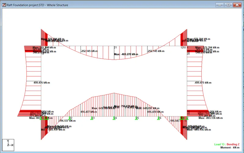
Normal Load Case + Temp (Accompanying).
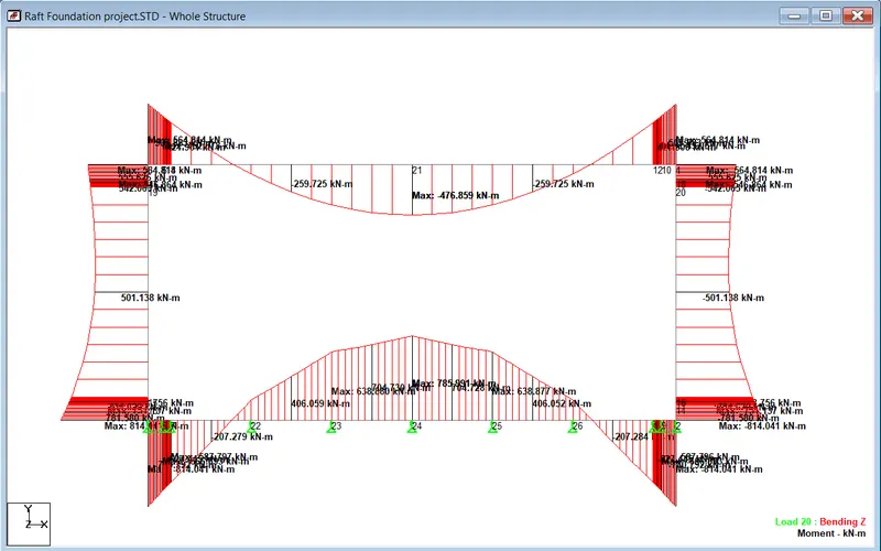
| FORCE SUMMARY (SLS) | |||||||||
| 5.2 Servicebility Limit State | |||||||||
| 5.2.1 Quas-Permanent Combination | LL model | SLS (quasi) | model | SLS (quasi) | model | SLS (quasi) | model | ||
| Live Load case (unfactored) from STAAD output |
Normal Load case (factored) from STAAD output |
Normal Load Case + Live Load |
Normal Load Case With Temperature Load (Accomp) |
Normal Load Case With Temperature + Live Load (Accomp) |
Normal Load Case With Temperature Load (Leading) |
Normal Load Case With Temperature + Live Load (Leading) |
Design Value |
||
| Moment kN-N | Moment kN-N | Moment kN-N | Moment kN-N | Moment kN-N | Moment kN-N | Moment kN-N | Moment kN-N | ||
| 21 | Mid top | 0 | |||||||
| Mid bot | 106.897 | 469.278 | 576.175 | 476.859 | 583.756 | 469.278 | 576.175 | 583.756 | |
| 4 & 6 | Support top | 123.904 | 572.364 | 696.268 | 564.814 | 688.718 | 572.364 | 696.268 | 696.268 |
| Support bot | 0 | ||||||||
| 17 & 19 | Outside | 123.904 | 572.395 | 696.299 | 584.818 | 708.722 | 572.395 | 696.299 | 708.722 |
| Inside | 0 | ||||||||
| 15 | Outside | 98.322 | 500 | 598.322 | 501.138 | 599.46 | 500 | 598.322 | 599.46 |
| Inside | 0 | ||||||||
| 13 & 2 | Outside | 77.13 | 803.137 | 880.267 | 814.011 | 891.141 | 803.137 | 880.267 | 891.141 |
| Inside | 0 | ||||||||
| 1 & 5 | Support top | 57.04 | 715 | 772.04 | 638.88 | 695.92 | 715 | 772.04 | 772.04 |
| Support bot | 72.74 | 803.137 | 875.877 | 814.041 | 886.781 | 803.137 | 875.877 | 886.781 | |
| 7 , 22 & 23 | top | 79.54 | 796.034 | 875.574 | 785.991 | 865.531 | 796.034 | 875.574 | 875.574 |
| bottom | 0 | ||||||||
Que 4) Do checks for ULS,SLS rare and quasi and present a hand calculation. & Also calculate the anchorage length of the bars and minimise the bars wherever you can.
| Sample Calculaion for Member 21 | ||||||
| Maximum BM under Basic combination | = | 759.00 | kN-m | 0.759 | 759000 | |
| Maximum SF | = | VNS | 446.00 | kN | ||
| Depth of member | = | D | 600.00 | mm | ||
| Width of the member | = | b | 1000.00 | mm | 1 | |
| Grade of Concrete Used | = | M35 | ||||
| Grade of Steel | = | Fe500 | ||||
| Charactristic strength of concrete | = | Fck | 35.00 | Mpa | ||
| Charactristic strength of steel | = | Fy | 500.00 | Mpa | ||
| Tensile strength of steel | = | Fctm | 2.80 | Mpa | ||
| Design yeild strenght of shear reinforcement | = | Fywd | 347.83 | Mpa | ||
| Partial material safety factor for concrete | = | gm | 1.50 | Basic | ||
| Partial material safety factor for steel | = | gs | 1.15 | Basic | ||
| Ultimate compressive strain in concrete | = | ϵcu3 | 0.00350 | Up to Fck | ||
| Modulus of elasticty of reinforcement of steel | = | Es | 200000.00 | Mpa | ||
| Modulus of elasticty of concrete | = | Ecm | 32000.00 | Mpa | ||
| Modular ratio | = | ɑe | 6.25 | |||
| Long term modular ration | = | ɑe | 12.50 | |||
| Ultimate tensile strain in the steel | = | ϵs | 0.00217 | |||
| Coefficient to consider the influence of the concrete strength | = | a | 0.67 | Cube | ||
| Factor | = | l | 0.80 | |||
| Factor | = | h | 1.00 | |||
| Design value of concrete compressive strength | = | fcd | 15.63 | |||
| Factor | = | Fav | 12.51 | |||
| Factor | = | β | 0.40 | |||
| Effective depth of member | = | d | 600.00 | mm | ||
| = | 540.00 | mm | 0.54 | |||
| = | Kav | 0.21 | ||||
| Limiting Neutral axis depth | = | Xlim | 333.10 | mm | ||
| = | X | 123.72 | mm | < | 333.1034 | |
| Required reinforcement | = | As | 3558.94 | mm2 | ||
| Provide | 12 | Nos | 20.00 | mm | 314 | |
| Provide renforcement | = | 3768.00 | mm2 | > | 3558.944 | |
| Netral axis deth | = | x | 130.99 | mm | < | 333.1034 |
| Xlim/d | = | 0.62 | ||||
| Rlim | = | 5.81 | ||||
| Effective depth required, | drequired | 361.40 | mm | |||
| Effective depth provided, | dprovided | 540.00 | mm | |||
| Shear design for member | ||||
| Vns | ||||
| Shear force VEd | = | 78633.14516 | > | 446 |
| Where v is a strenght reduction factor | = | 18.62903226 | ||
| Longitudinal force (NED) | = | 0 | ||
| Where | ||||
| K | = | 1.608580619 | ||
| Vmin | = | 0.374162246 | ||
| σcp | = | 0 | <= | 3.12666667 |
| ρ1 | = | 0.081 | <= | 0.02 |
| = | 141433.329 | |||
| = | ||||
| Sin2Ө | = | 0.176 | 312200 | 1772820 |
| SLS - Rare | ||||||
| Given Data | ||||||
| Model Calculation for Member | ||||||
| Maximum BM under Basic combination | = | 588.40 | kN-m | 0.588 | 588000 | |
| Maximum SF | = | VNS | 446.00 | kN | ||
| Depth of member | = | D | 600.00 | mm | ||
| Width of the member | = | b | 1000.00 | mm | 1 | |
| Grade of Concrete Used | = | M35 | ||||
| Grade of Steel | = | Fe500 | ||||
| Charactristic strength of concrete | = | Fck | 35.00 | Mpa | ||
| Charactristic strength of steel | = | Fy | 500.00 | Mpa | ||
| Tensile strength of steel | = | Fctm | 2.80 | Mpa | ||
| Design yeild strenght of shear reinforcement | = | Fywd | 347.83 | Mpa | ||
| Partial material safety factor for concrete | = | gm | 1.50 | Basic | ||
| Partial material safety factor for steel | = | gs | 1.15 | Basic | ||
| Ultimate compressive strain in concrete | = | ϵcu3 | 0.00 | Up to Fck | ||
| Modulus of elasticty of reinforcement of steel | = | Es | 200000.00 | Mpa | ||
| Modulus of elasticty of concrete | = | Ecm | 32000.00 | Mpa | ||
| Modular ratio | = | ɑe | 6.25 | |||
| Long term modular ration | = | ɑe | 12.50 | |||
| Ultimate tensile strain in the steel | = | ϵs | 0.00 | |||
| Coefficient to consider the influence of the concrete strength | = | a | 0.67 | Cube | ||
| Factor | = | l | 0.80 | |||
| Factor | = | h | 1.00 | |||
| Design value of concrete compressive strength | = | fcd | 15.63 | |||
| Factor | = | Fav | 12.51 | |||
| Factor | = | β | 0.40 | |||
| Effective depth of member | = | d | 600.00 | mm | ||
| = | 540.00 | mm | 0.54 | |||
| = | Kav | 0.16 | ||||
| Limiting Neutral axis depth | = | Xlim | 333.10 | mm | ||
| = | X | 93.55 | mm | < | 333.1034 | |
| Required reinforcement | = | As | 2690.91 | mm2 | ||
| Provide | 14 | Nos | 16 | mm | 200.96 | |
| Provide renforcement | = | 2813.44 | mm2 | > | 2690.908 | |
| Netral axis deth | = | x | 97.81 | mm | < | 333.1034 |
| Xlim/d | = | 0.62 | ||||
| Rlim | = | 5.81 | ||||
| Effective depth required, | drequired | 318.09 | mm | |||
| Effective depth provided, | dprovided | 540 | mm | |||
| SLS - Rare | ||||||
| Moment of Inertia of cracked section | = | 3438385003 | mm4 | |||
| Maximum compressive stress in concrete | = | 16.74 | < | 14.4 | Mpa | |
| Maximum tensile stress in steel | = | 472.943149 | < | 400 | Mpa | |
| SLS - Quasi | ||||||
| Given Data | ||||||
| Model Calculation for Member | ||||||
| Maximum BM under Basic combination | = | 583.76 | kN-m | 0.583 | 583000 | |
| Maximum SF | = | VNS | 446.00 | kN | ||
| Depth of member | = | D | 600.00 | mm | ||
| Width of the member | = | b | 1000.00 | mm | 1 | |
| Grade of Concrete Used | = | M35 | ||||
| Grade of Steel | = | Fe500 | ||||
| Charactristic strength of concrete | = | Fck | 35.00 | Mpa | ||
| Charactristic strength of steel | = | Fy | 500.00 | Mpa | ||
| Tensile strength of steel | = | Fctm | 2.80 | Mpa | ||
| Design yeild strenght of shear reinforcement | = | Fywd | 347.83 | Mpa | ||
| Partial material safety factor for concrete | = | gm | 1.50 | Basic | ||
| Partial material safety factor for steel | = | gs | 1.15 | Basic | ||
| Ultimate compressive strain in concrete | = | ϵcu3 | 0.0035 | Up to Fck | ||
| Modulus of elasticty of reinforcement of steel | = | Es | 200000.00 | Mpa | ||
| Modulus of elasticty of concrete | = | Ecm | 32000.00 | Mpa | ||
| Modular ratio | = | ɑe | 6.25 | |||
| Long term modular ration | = | ɑe | 12.50 | |||
| Ultimate tensile strain in the steel | = | ϵs | 0.00 | |||
| Coefficient to consider the influence of the concrete strength | = | a | 0.67 | Cube | ||
| Factor | = | l | 0.80 | |||
| Factor | = | h | 1.00 | |||
| Design value of concrete compressive strength | = | fcd | 15.63 | |||
| Factor | = | Fav | 12.51 | |||
| Factor | = | β | 0.40 | |||
| Effective depth of member | = | d | 600.00 | mm | ||
| = | 540.00 | mm | 0.54 | |||
| = | Kav | 0.16 | ||||
| Limiting Neutral axis depth | = | Xlim | 333.10 | mm | ||
| = | X | 92.69 | mm | < | 333.1034 | |
| Required reinforcement | = | As | 2666.20 | mm2 | ||
| Provide | 14 | Nos | 16.00 | mm | 200.96 | |
| Provide renforcement | = | 2813.44 | mm2 | > | 2666.204 | |
| Netral axis deth | = | x | 97.81 | mm | < | 333.1034 |
| Xlim/d | = | 0.62 | ||||
| Rlim | = | 5.81 | ||||
| Effective depth required, | drequired | 316.74 | mm | |||
| Effective depth provided, | dprovided | 540.00 | mm | |||
| SLS - Quasi | ||||||
| Moment of Inertia of cracked section | = | 6876672199 | mm4 | |||
| Maximum compressive stress in concrete | = | 8.30277967 | < | 14.4 | Mpa | |
| Maximum tensile stress in steel | = | 469.221083 | < | 400 | Mpa | |
| Equivalent diameter Фeq | = | 18.2222 | mm | |||
| Where spacing of bonded reinforcement with in the | <= | 275 | ||||
| tension zone | ||||||
| Wk | = | 0.63190887 | < | 0.3 | mm | |
| maximum cracking spacing, Sr max | = | 335.159615 | ||||
| Rr.eff | = | 0.0188 | ||||
| (esm - ecm) | = | 0.0018854 | 0.001408 | |||
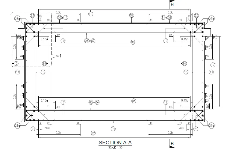
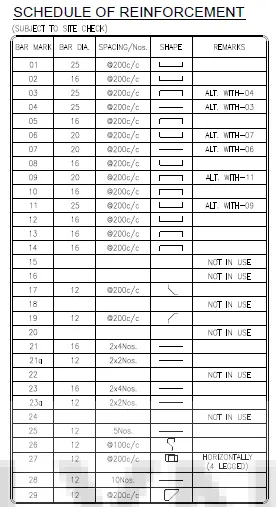
Que 6) Draw rebars to the scale and therefore calculate the kg/cumec of the base slab.
Reinforcement Detail.