Internal flow simulation in a pipe with an inlet Reynolds number of 100,1000 and 10,000.

Aim:

Run a pipe flow simulation with an inlet Reynolds number of 100,1000 and 10,000.

For each of these cases do the following

1. To Place line probes at 95%, 90% and 85% of the pipe length.
2. Also Place three-line probes near the inlet length of the pipe.
3. Compare the velocity profile at each of these locations.

Overview:

About the software

Flow Simulation is a CFD software that is completely build inside of solidWorks. This is its main advantage since we don’t have to do any file transfer or save an intermediate file type to do the analysis, it happens in the same interface where we design most of the CAD geometry. And if need to make any design changes we switch tab to alter design, based om analysis results. While CFD and equation that run Flow simulation in the background are complicated, simple user interface makes it easy to use. We can also compare results of different scenarios and evaluate performance and make design decisions. Furter we can optimize the performance of our design through the results that we get. And most importantly we can also simulate industry standard tests to cut cost and save time.

With Flow Simulation we can perform following Analysis:

• Internal flow analysis which involves tubes, constriction, valves etc
• External flow analysis to check Aerodynamics or to simulate virtual wind tunnel
• Laminal and Turbulent
• Heat Transfer
• Analysis involving rotating components, compressible and non-Newtonian fluid
• Steady state or transient Time dependent analysis
• Free Surface flow
• Fluid mixing

Internal flow

In internal flow, the conduit is completely filled with the fluid, and the flow is driven primarily by a pressure difference. Liquid or gas flow through pipes or ducts is commonly used in heating and cooling applications and fluid distribution networks. The fluid in such applications is usually forced to flow by a fan or pump through a flow section. We pay particular attention to friction, which is directly related to the pressure drop and head loss during flow through pipes and ducts. The pressure drop is then used to determine the pumping power requirement

Most fluids, especially liquids, are transported in circular pipes. This is because pipes with a circular cross section can withstand large pressure differences between the inside and the outside without undergoing significant distortion. Noncircular pipes are usually used in applications such as the heating and cooling systems of buildings where the pressure difference is relatively small, the manufacturing and installation costs are lower, and the available space is limited for ductwork

The fluid velocity in a pipe changes from zero at the wall because of the no-slip condition to a maximum at the pipe centre. In fluid flow, it is convenient to work with an average velocity Vavg, which remains constant in incompressible flow when the cross-sectional area of the pipe is constant.

The primary consequence of friction in fluid flow is pressure drop, temperature rise due to frictional heating is usually too small to warrant any consideration in calculations and thus is disregarded.

Laminar and Turbulent Flow

Laminar, characterized by smooth streamlines and highly ordered fluid motion. Turbulent flow is characterized by velocity fluctuations and highly disordered motion. The transition from laminar to turbulent flow does not occur suddenly; rather, it occurs over some region in which the flow fluctuates between laminar and turbulent flows before it becomes fully turbulent.

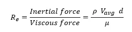
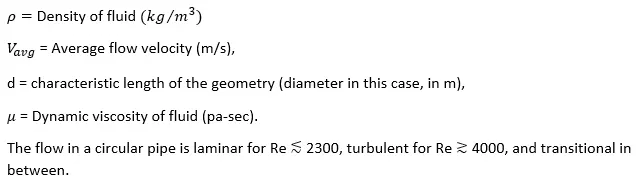
After exhaustive experiments in the 1880s, Osborne Reynolds discovered that the flow regime depends mainly on the ratio of inertial forces to viscous forces in the fluid. This ratio is called the Reynolds number and is expressed for internal flow in a circular pipe as

Steps Taken:

• Creating pipe model (all dimensions in mm):

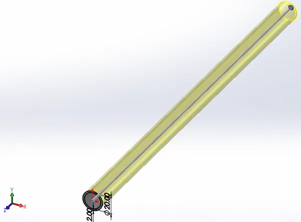
Length of pipe =450mm

• Putting Line probe at 95%, 90%, and 85% of pipe length i.e., at 427.5mm, 405mm and 382.5mm from origin respectively.

Three-line probes are also placed near inlet of the pipe to get the whole picture of velocity profile.

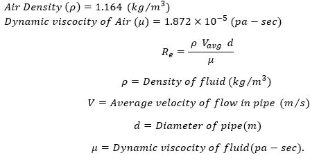
• Calculating velocity of flow with respect to Reynolds number ).

Working fluid = Air

Properties of Air at 1 atm pressure and 30 °C:

• For Reynolds number 100

• For Reynolds number 1000

• For Reynolds number 10000

• Using ‘Flow Simulation’ tab:

• Creating lids
• Setting up Flow simulation Project using ‘Analysis Wizard’

It asks us a series of questions that sets up majority of our analysis. In Analysis wizard we choose type and analysis and select fluid from extensive database.

Selecting Unit system as SI.

Analysis type = Internal

Turing Gravity on in Y-component = -9.81 m/s^2

Fluid = Air

Flow type = Laminar and Turbulent

In Thermodynamic Properties, select Temperature = 303.15 K, Pressure = 101325 Pa

• After setting up wizard we have couple of steps to take,
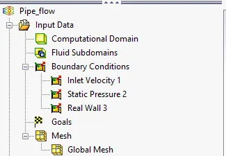
• Specifying the boundary conditions

At inlet, input inlet velocity (0.0804 , 0.804 & 8.04 ).

At outlet, specify atmospheric pressure at the outlet.

Specify the inner surface of the pipe as, Real wall.

• Providing goals – reasons for doing analysis
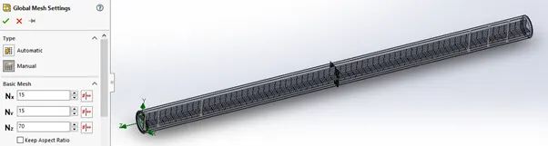
• Change mesh size to a finer mesh for more accurate results.

• Results & Observations: Velocity profile plots at various locations for 3 flow velocity conditions.

1. For, Velocity = 0.0804 m/s (Laminar Flow)

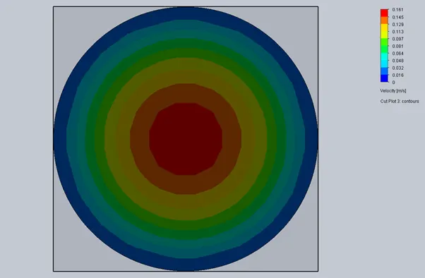
Following show the variation of velocity in the pipe using a cut plot for the mid-section of the pipe from front plane.

It also shows the graph for velocity profile at different sections viz. 4mm, 20mm, 70mm, 382.5mm, 405mm & 427.54mm form the origin.

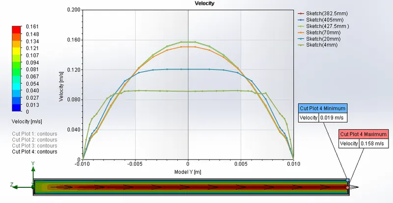
• From the cut-plot we can clearly see the velocity gradient marked by different colours. The region in contact with the wall are marked with blue depicting zero velocity and as we move towards the centre of the pipe the flow velocity increases and reaches to maximum at the centre (marked by red).

This is because of the no-slip condition, the fluid particles in the layer in contact with the wall of the pipe come to a complete stop (marked by blue colour). This layer also causes the fluid particles in the adjacent layers to slow down gradually as a result of friction. To make up for this velocity reduction, the velocity of the fluid at the midsection of the pipe has to increase to keep the mass flow rate through the pipe constant. As a result, a velocity gradient develops along the pipe.

This also explains, why in spite our inlet velocity being 0.0804 m/s maximum velocity we get in the pipe is around 0.161 .

• From the plot it is clear that maximum velocity in the pipe is around 0.161 m/s . Which can also be proved from the formula of velocity profile,

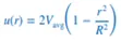
by putting r = 0. u(max) = 2 * Vavg = 2 * 0.0804 = 0.1608 m/s.

• The region of the flow in which the effects of the viscous shearing forces caused by fluid viscosity are felt is called the velocity boundary layer or just the boundary layer.

• Velocity Profile at different lengths across the pipe.

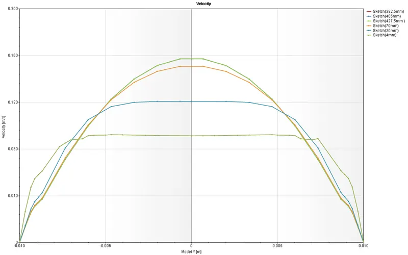
In the above graph the x-axis represents the Diameter of the pipe whereas y-axis, the velocity of fluid inside the pipe.

• Since this is a case of laminar flow, the velocity profile in the fully developed region is parabolic.
• The plot line for 4mm, 20mm and 70mm shows developing velocity profile, where as the velocity profile for 382.5mm, 405mm and 427.5mm (all superimposed in top most green parabolic curve) represents fully developed velocity profile.
• The region from the pipe inlet to the point at which the velocity profile is fully developed is called the hydrodynamic entrance region, and the length of this region is called the hydrodynamic entry length . Here, is likely to lie in between 0 – 100mm.

It can be proved from the formula, ,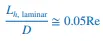

• The region beyond the entrance region in which the velocity profile is fully developed and remains unchanged is called the hydrodynamically fully developed region. Here, hydrodynamically fully developed region is likely to likely to lie in between 100mm to 450mm.
• It can also be inferred from the graph that at either end of the pipe (i.e., at the wall) the velocity is zero due to no-slip condition. The velocity increases gradually, and reaches its peak at the core where the frictional effects are negligible and the velocity remains essentially constant in the radial direction.
• Hence, velocity increases in a pipe flow in 2 ways, first, as we move from inlet to outlet and as we move from boundary wall to the centre of the pipe. But it should be noted that the discharge or the mass flow rate at inlet and outlet remains the same.
• Cut plot of pipe from front view at 427.5mm from inlet, to show the radial velocity variation in hydrodynamically fully developed region.

2. For, Velocity = 0.804 m/s (Laminar Flow)

Following show the variation of velocity in the pipe using a cut plot for the mid-section of the pipe from front plane.

It also shows the graph for velocity profile at different sections viz. 4mm, 20mm, 70mm, 382.5mm, 405mm & 427.54mm form the origin.

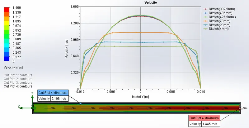
• It can be seen from the graph that at boundary wall the velocity is nearly zero and reaches maximum at the pipe centre i.e., 1.446 m/s.
• Velocity in the pipe increases in 2 ways, first, as we move from inlet to outlet and as we move from boundary wall to the centre of the pipe. But it should be noted that the discharge or the mass flow rate at inlet and outlet remains the same.

• Velocity Profile at different lengths across the pipe.

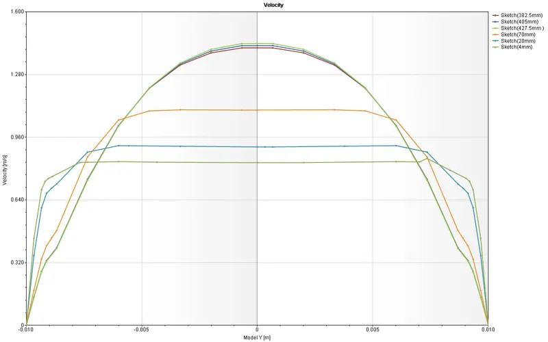
In the above graph the x-axis represents the Diameter of the pipe whereas y-axis, the velocity of fluid inside the pipe.

• The plot line for 4mm, 20mm and 70mm shows developing velocity profile, whereas the velocity profile for 382.5mm, 405mm and 427.5mm represents velocity profile reaching fully developed velocity profile.
• The region from the pipe inlet to the point at which the velocity profile is fully developed is called the hydrodynamic entrance region, and the length of this region is called the hydrodynamic entry length .

It can be proved from the formula, ,

So, hydrodynamic entrance region lies in between 0 – 1000mm.

• The region beyond the entrance region in which the velocity profile is fully developed and remains unchanged is called the hydrodynamically fully developed region. Here, hydrodynamically fully developed region is likely to lie beyond 1000mm pipe length.
• Cut plot of pipe from front view at 427.5mm from inlet, to show the radial velocity variation in hydrodynamically fully developed region.

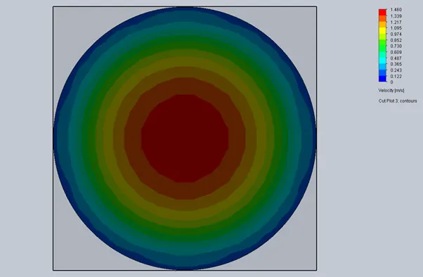
3. For, Velocity = 8.04 m/s (Turbulent Flow)

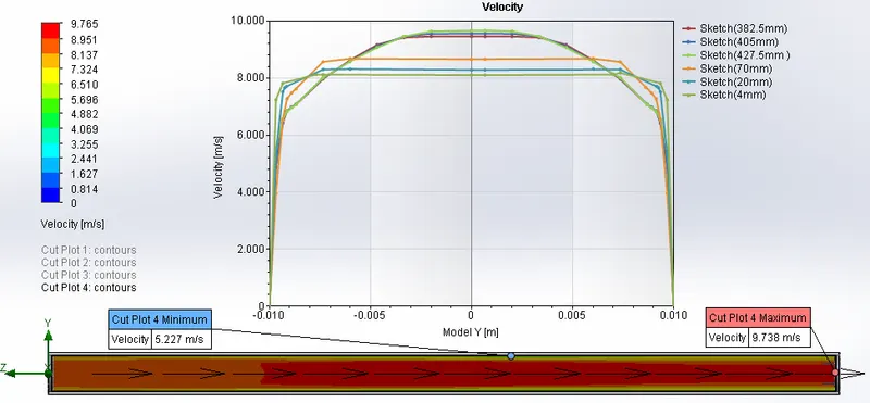
• Velocity Profile at different lengths across the pipe.

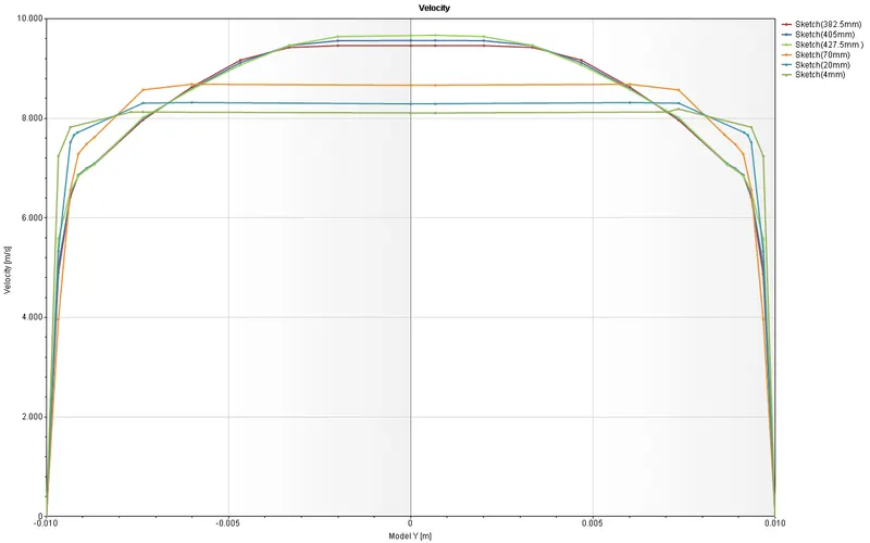
In the above graph the x-axis represents the Diameter of the pipe whereas y-axis, the velocity of fluid inside the pipe.

• The plot line for 4mm, 20mm and 70mm, 382.5mm, 405mm shows developing velocity profile, whereas 427.5mm depicts fully developed velocity profile.
• Since, this is a case of turbulent flow the velocity profile here is much flatter (or fuller) due to eddy motion and more vigorous mixing in the radial direction.
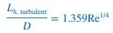
• Hydrodynamic entry length for turbulent flow is approximated as, ,

Hydrodynamic entrance region lies in between 0 - 271.8mm.

• Hydrodynamically fully developed region lies between 271.8 – 450mm.
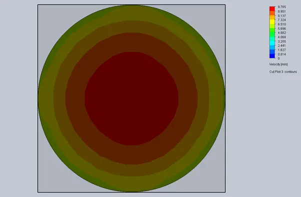
• Cut plot of pipe from front view at 427.5mm from inlet, to show the radial velocity variation in hydrodynamically fully developed region.

References:

FLUID MECHANICS (FUNDAMENTALS AND APPLICATIONS) by Yunus Cengel and John Cimbala.