Aim-Modelling and analysing the Wide Open Throttle response for EV.

Objectives-

1. To calculate the ratio of hill-climbing power required by fully loaded TATA Ultra Truck to the half-loaded one.
2. To find the minimum length of flyover planned to be constructed on a national highway. Keeping in mind about the gradeability for trucks, considering the minimum height at the summit should be 5.5 meters.
3. To prepare a new drive cycle excel file for the model and also include a hill-climbing angle to it. Revise the model file Driver_Glider.slx and comment on the results.
4. To model the WOT (Wide Open Throttle) response of GM EV1 car. Compare it with the official figures of the performance of a real vehicle. Prepare a table showing variation in acceleration time with a 5% change in vehicle parameters.

Hill Climbing Power of TATA T.16 ULTRA | Day Variant | CAB –

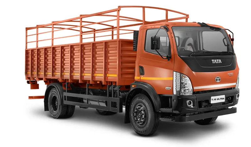
Specifications- https://light-trucks.tatamotors.com/pdf/t16-ultra.pdf

Power Ratio Excel Calculator

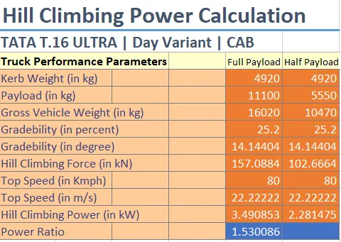
Minimum Length of the flyover-

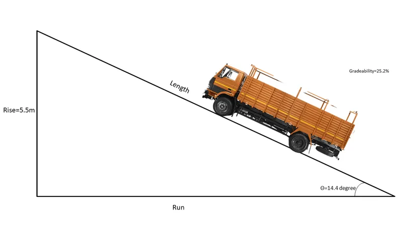
Here, we know

`"rise"=5.5m`

`theta=14.4^o`

as the gradeability of TATA Ultra T.16 is 25.2%.

now,Drive Cycle file

`"rise"/"run"=tan(theta)`

`5.5/"run"=tan(14.4)`

`5.5/"run"=0.2568`

`"run"=5.5/0.2568`

`"run"=21.41m`

Thus, the minimum length of the flyover needs to be atleast 21.41m so that vehicles are able to climb the flyover.

Revised Drive cycle for the driver_glider.slx model-

Drive Cycle-

Drive cycle file

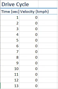
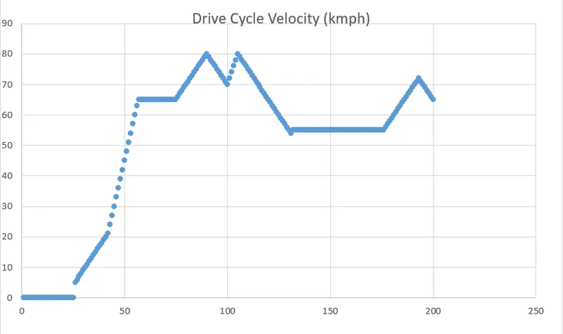
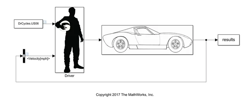
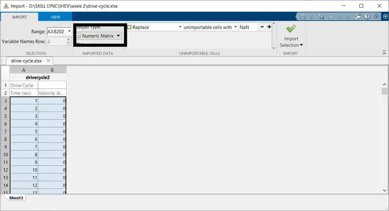
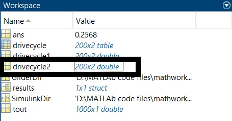
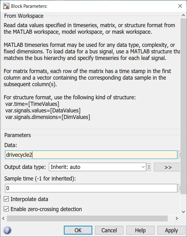
The default drive cycle is changed with the revised custom drive cycle.

Driver Model-

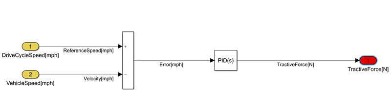
It is a just a PID controller that minimises the error in between the Input drive cycle provided and the actual speed that the vehicle is incorporating.

Vehicle Model-

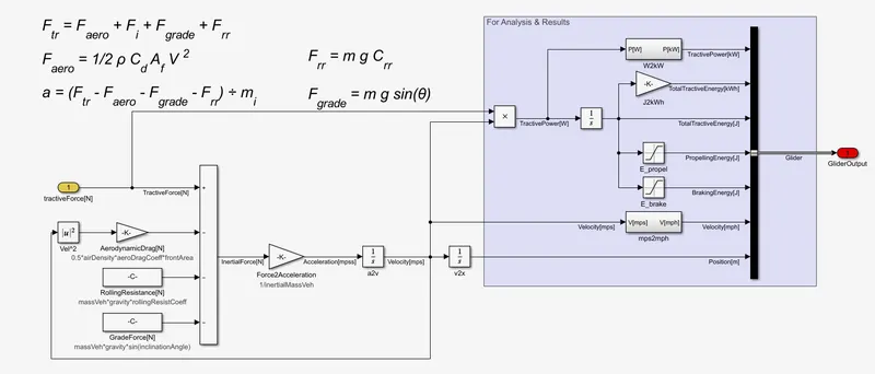
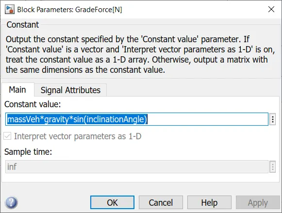
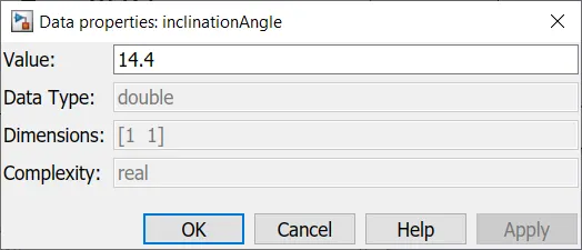
To change the grade we changed the value of GradeForce constant block.

Revised Model Output-

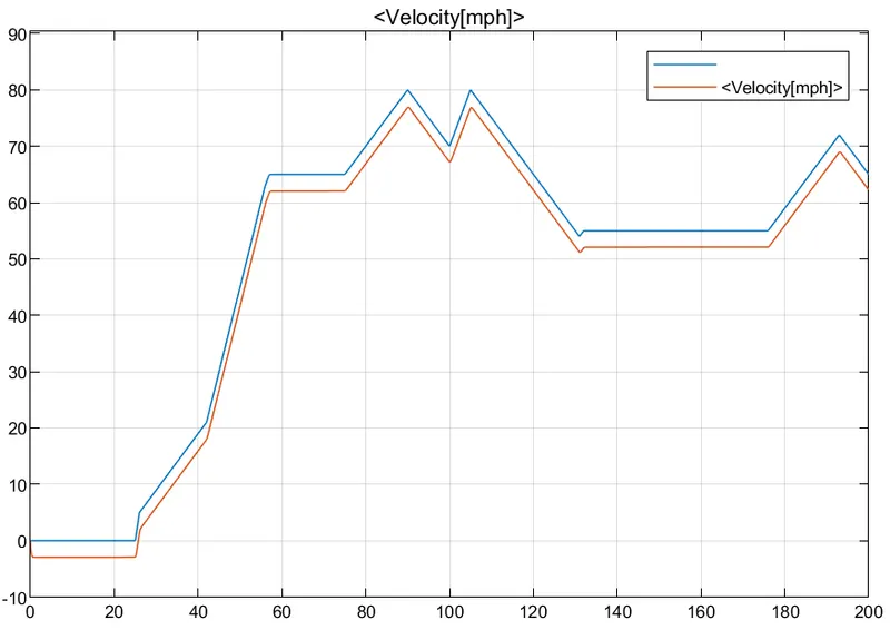
From the inspection of the graph obtained above we can clearly see that the tractive force is insufficient to track the driving cycle if the grade is 14.4 degree.

WOT (Wide Open Throttle) response of GM EV1 car-

Specifications-

Vehicle Mass (with 70 kg passenger)	1540 kg
Drag Coefficient	0.19
Coefficient of rolling resistance	0.0048
Motor speed	12000 RPM
Tyre radius	0.30 m
Gear ratio	11
Motor torque	140 Nm
Angular velocity	733 rad/s
Efficiency of drive	0.95
Frontal Area	1.8 m^2
Constant power	102 kW
Critical velocity	19.8 m/s

Calculations-

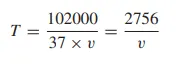
Motor torque characteristic equation for GVEV1 is given by-

we know that,

Tractive force can be expressed as

Below critial velocity we can take `T=T_(max)`

substituting values we get

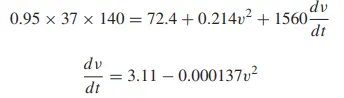
When the vehicle reaches the critical velocity-

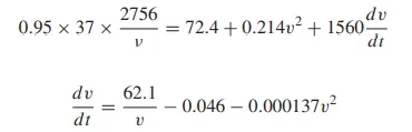
The above two differential equations are now put in finite differences form

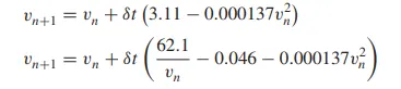
MATLAB Script-

%% =============GMEV1 - Wide open throttle response========================
t=linspace(0,50,501);                % 0 to 50 s, in 0.1 s steps
vel=zeros(1,501);                    % 501 readings of velocity
d=zeros(1,501);                      % Array for storing distance travelled
dT=0.1;                              % 0.1 second time step
for n=1:500

if vel(n)<19.8                       % Torque constant till this point
vel(n+1)= vel(n) + dT*(3.11 - (0.000137*(vel(n)^2)));
elseif vel(n)>=35.8
vel(n+1)=vel(n);
else
vel(n+1)=vel(n)+dT*((62.1/vel(n))-0.046-(0.000137*(vel(n)^2)));
end
end
vel=vel.*3.6;                       % Multiply by 3.6 to convert m/s to kph
plot(t,vel);
xlabel('Time / seconds');
ylabel('Velocity / kph');
title('Full power (WOT) acceleration of GMEV1');

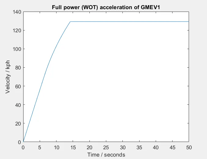
This script executes three conditions-

• when the velocity is less than 19.8m/s

• vel(n+1)= vel(n) + dT*(3.11 - (0.000137*(vel(n)^2)));

• when the velocity is greater than 35.8m/s

• vel(n+1)=vel(n);

• when the velocity is between 19.8m/s to 35.8m/s

• vel(n+1)=vel(n)+dT*((62.1/vel(n))-0.046-(0.000137*(vel(n)^2)));

Specifications (increased 5%)-

Property	Original	5% increased
Vehicle Mass (with 70 kg passenger)	1540 kg	1677 kg
Drag Coefficient	0.19	0.1995
Coefficient of rolling resistance	0.0048	0.0050
Motor speed	12000 RPM	12600
Tyre radius	0.30 m	0.3150
Gear ratio	11	11.5500
Motor torque	140 Nm	147
Angular velocity	733 rad/s	769.6500
Efficiency of drive	0.95	0.9975
Frontal Area	1.8 m^2	1.8900
Constant power	102 kW	107.1000
Critical velocity	19.8 m/s	20.7900

MATLAB Script-

%% =============GMEV1 - Wide open throttle response========================
t=linspace(0,50,501);                % 0 to 50 s, in 0.1 s steps
vel=zeros(1,501);                    % 501 readings of velocity
d=zeros(1,501);                      % Array for storing distance travelled
dT=0.1;                              % 0.1 second time step
for n=1:500

if vel(n)<19.8                       % Torque constant till this point
vel(n+1)= vel(n) + dT*(3.11 - (0.000137*(vel(n)^2)));
elseif vel(n)>=35.8
vel(n+1)=vel(n);
else
vel(n+1)=vel(n)+dT*((62.1/vel(n))-0.046-(0.000137*(vel(n)^2)));
end
end
%vel=vel.*3.6;                       % Multiply by 3.6 to convert m/s to kph


%% ===========GMEV1 - Wide open throttle response (5% changed)=============
t2=linspace(0,50,501);               % 0 to 50 s, in 0.1 s steps
vel2=zeros(1,501);                   % 501 readings of velocity
d=zeros(1,501);                      % Array for storing distance travelled
dT=0.1;                              % 0.1 second time step
for n=1:500

if vel2(n)<20.79                     % Torque constant till this point
vel2(n+1)= vel2(n) + dT*(3.1195 - (0.00069605*(vel2(n)^2)));
elseif vel2(n)>=37.59
vel2(n+1)=vel2(n);
else
vel2(n+1)=vel2(n)+dT*((59.3994/vel2(n))-0.0485-(0.00069605*(vel2(n)^2)));
end
end
%vel2=vel2.*3.6;                     % Multiply by 3.6 to convert m/s to kph

plot(t,vel,t2,vel2);
xlabel('Time / seconds');
ylabel('Velocity / kph');
title('Full power (WOT) acceleration of GMEV1');

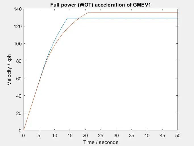
From the inspection of the above graph we can say that the vehicle velocity remains constant after reaching the maximum value

• With Original paramters- velocity= 35.8 m/s or 128.88 km/hr
• With Changed parameter- velocity= 37.59 m/s or 135.324 km/hr