Mixing efficiency

1. Introduction:

Mixing Tee is one of the simplest and cost effective method to mix the two fluids having different temperature and flow rate. The prime areas of application are air conditioning units, petrochemical industries and pharmacuetical industries. The prime objective of present steady state CFD analysis using Ansys fluent is to study the performance of mixing tee within which the hot and cold fluid (air) is mixed entering with different velocity at their respective inlets. The hot fluid is entering at a temperature of 36 deg celsius while the cold fluid is entering with a temperature of 19 degree celsius. Two geometrical cases are considered in this study i) Long mixing tee section ii) short mixing tee section, whiile the momentume ratio for both the cases is kept at a value of 2 and 4. Finally it has to be determined how the geometry, turbulence model and momentum ratio will affect the outlet temperature of the fluid.

2. Geometry Set up:

The initial and first step was to create the geometry in space claim or any other CAD package. After creating or importing the geometry of mixing tee in space claim the next step is to clean up the geometry by supressing the non fluid region. Once the geometry is cleaned up now the geometry is ready for meshing.

3. Meshing:

Meshing is the process of dividing the domain of intrest in to number of small elements having different shapes. Now for the present mixing tee geometry it is better to use tetrahedron mesh.Most of the features in meshing will be taken care by ansys fluent itself.

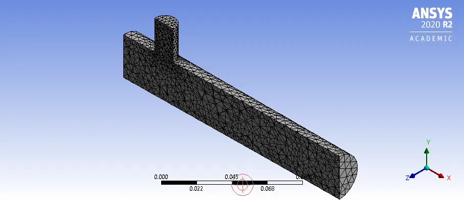
Figure 1. Meshing

After generating the mesh of required element size as shown in the above figure 1. Next step is to name the different regions of the geometry such as inlet, outlet and walls.The name selection is necesssary part as it helps to define the boundary conditions to be assigned.

The below table 1 shows the details of mesh used for both the cases of mixing tee.

Case No	Mesh Type	Geometry Type	No of nodes	No of Elements
Case 1	Tetrahedron	Long Mixing Tee	3448	15483
Case 2	Tetrahedron	Short Mixing Tee	2827	12728

4. Setup:

After completeing the meshing process the next step isto define the physics of the geometry and methods used for obtaining the final required solution. The mixing tee problem is having simple geometry hence it is solved for steady state condition with hybrid initilization method. The flow is assumed to be viscous and turbulent. Hence to catch the turbulent behaviour of the fluid diffrent methods are available and for present problem the K-epsilon and K-omege model were used. Out of these two methods the most suitable method which gives better stability is choosen. The following table 2 shows the physical parameters used to solve the mixing tee problem.

Table2. Physical Parameters

Case No	Geometry Type	Momentum Ratio (MR)	Inlet Velocity (x)	Inlet Velocity (y)	Inlet Temp (x)	Inlet Temp (y)	Outlet (x)
Case 1	Mixing Tee Long	a. 2 b. 4	3m/s	a. 6m/s b. 12m/s	36 deg celsius	19 deg celsius	Atm pressure
Case 2	Mixing Tee short	a. 2 b. 4	3m/s	a. 6m/s b. 12m/s	36 deg celsius	19 Deg celsius	Atm Prewssure

Aftrer performing the physical set up the solution is initialized by using hybrid initilization method once the initilization is done next the solution is run for different number of iterations. The process of iteration repeated until a converged solution is obtained.

The convergence is the process which is used ti identify that the obtained solution for the given problem has reached a stedy state.

The following figure 2 shows the residual graph obtained for both the cases of mixing tee and from these residual values one can easily come to know that the solution is converged or not.

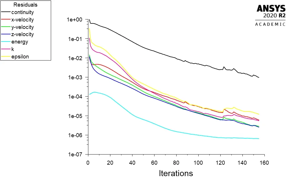
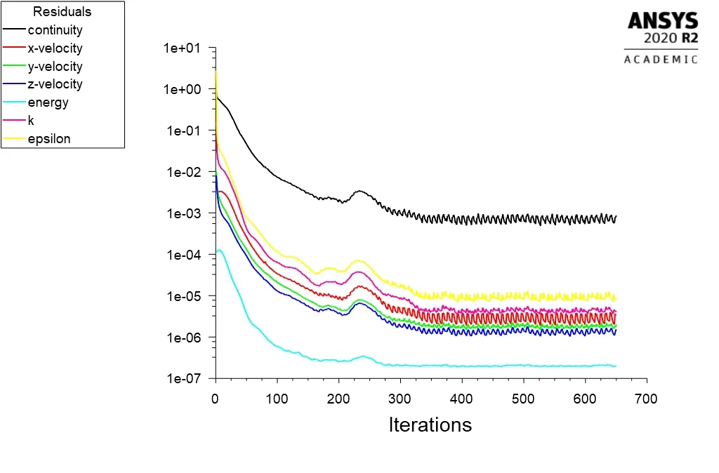
Figure 2. Residual Plots for mixing tee.

From above figure 2 it is clearly observed that the residual of different parameters shown the steady behavoiur after some number of iterations and in this case the number of iterations are around 250. After which the nature of all the residual variable ramin same which shows that ateady atate has been achieved. Hence the criteria for convergence has been reached.

5. Results:

The post processing of mixing tee is performed in order to plot and analyse the different variables and parameters used in the study. The following figures shows the contour plots for temperture and velocity in both the cases of mixing tee.

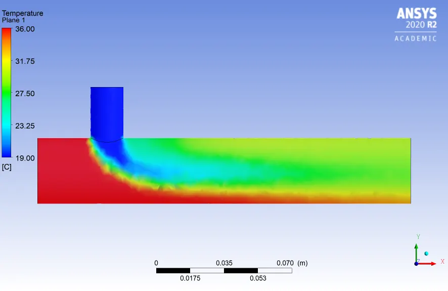
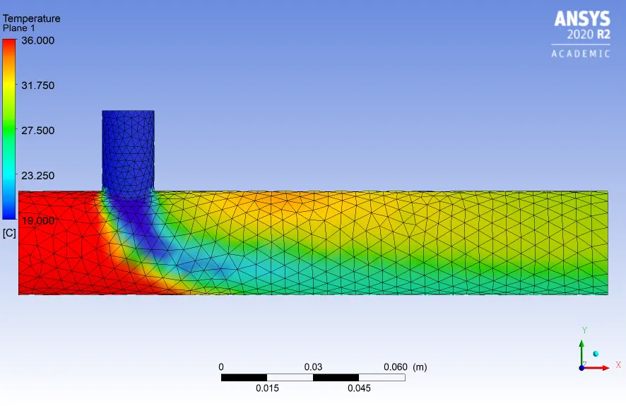
Figure 3a Figure 3b

Figure 3. Temperature contour Mixing Tee (Short) a. MR=2, b. MR=4

The velocity contours for mixing tee of short lenght geometry is as shown below in the figure 4.

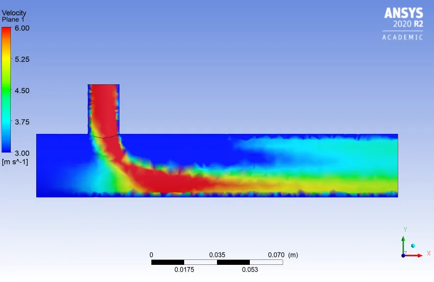
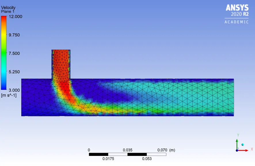
Figure 4a. MR=2 Figure 4b. MR=4

Figure 4. Velocity contours Mixing tee (short) a. MR=2, b. MR=4

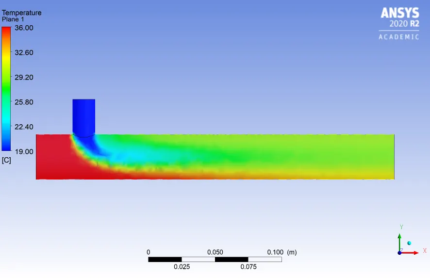
The figure 5 below shows the temperature and velocity contours for long mixing tee.

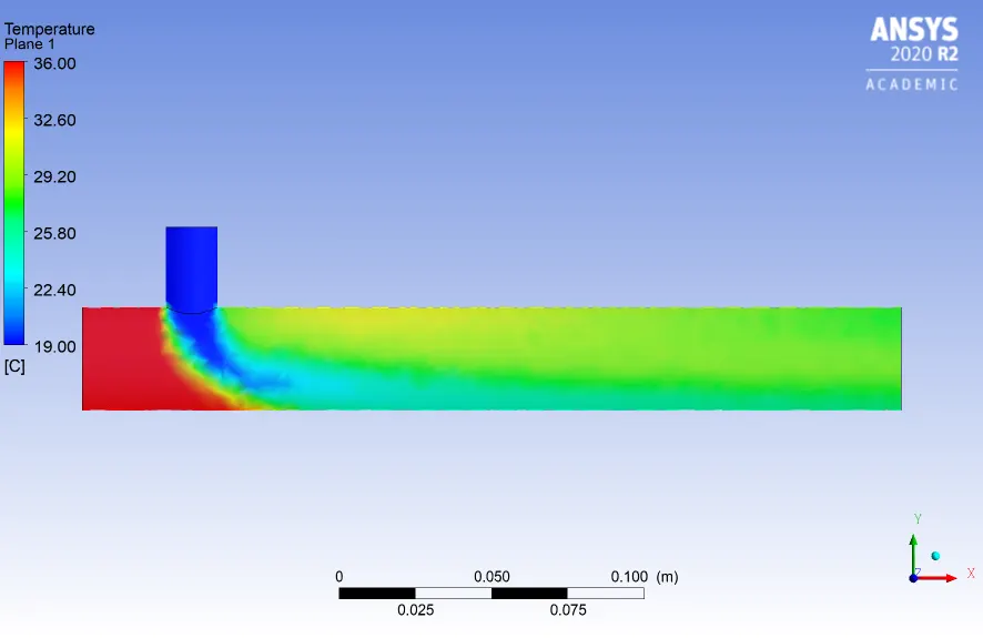
a.MR=2 b. MR=4

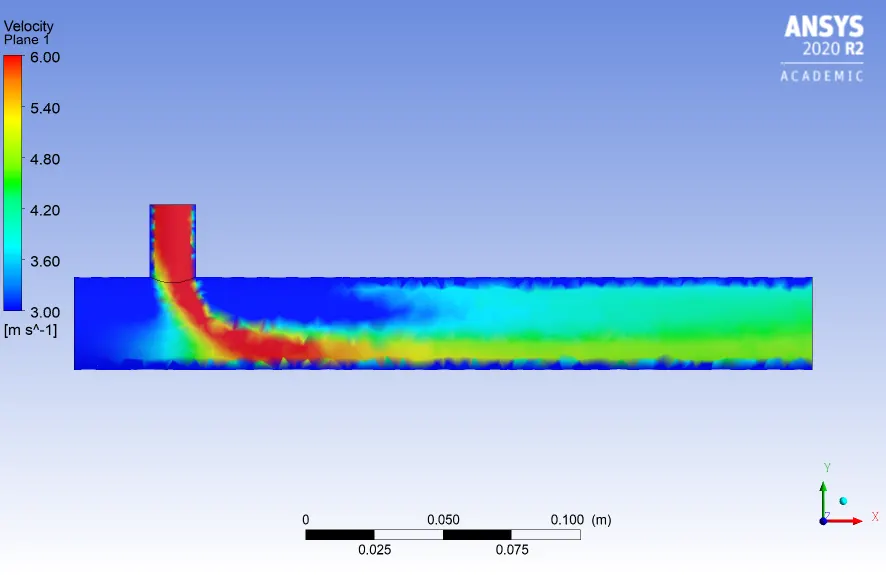
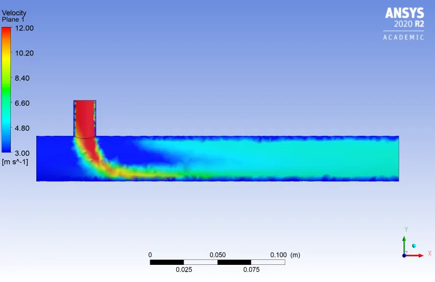
c. MR=2 d. MR=4

Figure 5. a. Temp Contour MR=2, b. Temp Contour MR=4, c. Velocity contour MR=2. d. Velocity contour MR=4

6. Conclusions:

From the above obtained results the following conclusions are obtained

1. With increse in the momentum ratio the temperature of mixed fluid will drop sufficiently at the outlet section.

2. The momentum ratio of 4 is more effective in reducing the temperature in both the cases of micing tee compare to MR of 2.

3.The mixing tee with short lenght proves to be more effective in controlling the outlet temperature of the fluid as compare to that of long length mixing tee.

4. The chances of back flow is more in case of MR=4 compare to MR=2.

5. The maximum devaition in the temperature of the fluid occurs at MR=2 and minimum deviation occurs at MR=4. and among mxing tee cases the maximum temperature deviation is observed in short lenght mixing tee for MR=2 and minimum temperature deviation is oberved in case of long mixing tee for MR=4.

6. It is better to use short length mixing tee with high momentum ratio but at the cost of pumping power.